Growth in Variant of Concern
Written in May 2021
Added note in July 2021: the point of the second section is to try to get a modelling advantage, in terms of better accuracy and less lag, by combining two different things, the variant counts and the total case counts. The assumption is that the variant counts are only a sample, a subset, of the total case counts, and they are delayed by around two weeks, so "total case counts" is bringing something extra to the party. The method's advantage can only last as long as there are a significant number of each variant type, but by July almost all cases in the UK were Delta so this method becomes similar to standard binomial (or, in general, multinomial) fitting of the variant types.
The objective here is to try to understand to what extent the variant of concern B.1.617.2 (first found in India, now known as Delta) is growing in the UK, both in its own terms and in comparison to B.1.1.7 (first found in Kent, now known as Alpha). Different methods seemed to be giving different answers and this is an attempt to reconcile them.
Most indicators considered here suggest a substantial transmission advantage of B.1.617.2 over B.1.1.7, estimated as about 60-70% country-wide, or an extra growth rate of about 10-11% per day, though possibly lower in certain places like London. Here "transmission advantage" is here taken to mean the extra biological transmissibility of B.1.617.2 together with any immune-escape advantages it may have at the current level of vaccinations and past infections. In other words, "transmission advantage" is taken to mean $$R_t(\text{B.1.617.2})/R_t(\text{B.1.1.7})$$, and not, for example, $$R_0(\text{B.1.617.2})/R_0(\text{B.1.1.7})$$. The model used here finds typical R numbers of 0.9 for B.1.1.7 and 1.5 for B.1.617.2, though they vary around the country and are notably lower in some areas. In particular, Bolton seems to have crushed the outbreak, presumably by means of intensive "surge" tactics, and Wales, without any particular country-wide surge tactics, has a considerably lower virus growth rate than the rest of the UK, maybe in part due to the significantly higher vaccination levels in that nation.
This analysis is predicated on the idea that there is a single multiplicative constant, the ratio of the (time-varying) R-numbers for B.1.617.2 and B.1.1.7, that is independent of suppression measures or immunity. This seems plausible as an approximation, though it is not biologically guaranteed.
Estimating transmission advantage using variant counts only
One method is to compare counts of B.1.617.2 with counts of B.1.1.7 (first found in Kent/UK, dominant in the UK from February to early May) on two or more occasions and take cross ratios. This method has the advantage that some of the uncertainties and variabilities will naturally cancel out. For example, if people change their work patterns to working from home then that will slow down the transmission of both variants, so the comparison between them will hopefully be relatively unaffected. However, there are still some residual sources of uncertainty, as discussed below.
Let's say $$A$$ and $$B$$ cases of variants V1 and V2 respectively were detected during some (short) time period, and then 5 days later $$C$$ and $$D$$ cases of V1 and V2 were detected. We'll use the simplified assumptions that the growth rates of the two variants differ by a constant, that their generation times are the same, and that the generation times can be approximated by a constant, 5 days. In that case we'd expect $$C=Q_0sA$$ and $$D=R_0sB$$, where $$Q_0$$ and $$R_0$$ are the basic reproduction numbers of variants V1 and V2, and $$s$$ represents overall susceptibility, which includes the proportion of the population that are still biologically susceptible to catching the virus together with any behavioural modifications that might alter the propensity for disease to spread. We see the cross ratio, $$AD/(BC)$$ is equal to $$R_0/Q_0$$, the extra transmissibility, while $$s$$ is cancelled out. Working out $$R_0$$ or $$Q_0$$ individually is not possible from these numbers, but this ratio comparison between them is relatively easy.
Note that if there are two subpopulations with the same susceptibility, $$s$$, then you may as well lump them together as the cross ratio between $$A+A'$$, $$B+B'$$, $$Q_0sA+Q_0sA'$$ and $$R_0sB+R_0sB'$$ is still $$R_0/Q_0$$. We shall discuss the effect of aggregating subpopulations of different susceptibilities below, but first let's see what we get with counts aggregated to UK level.
To do a calculation all we need is the pair of counts at two times. There are several possible data sources for the UK, including The Wellcome Sanger Institute, COG-UK or weekly government updates. This is from the UK-wide counts in COG-UK's metadata file and was generated with this program:
| Week ending date | B.1.1.7 | B.1.617.2 | Est'd transmission advantage from previous week |
|---|---|---|---|
| 2021-04-17 | 7446 | 172 | |
| 2021-04-24 | 7117 | 450 | 105% (81% - 133%) |
| 2021-05-01 | 6134 | 846 | 75% (60% - 90%) |
| 2021-05-08 | 4918 | 1584 | 83% (72% - 96%) |
| 2021-05-15 | 3920 | 2629 | 69% (60% - 78%) |
(Note that these transmissibility numbers are due to be refined below and shouldn't be taken as the best estimate.)
Given four numbers $$A$$, $$B$$, $$C$$, $$D$$ arranged like this:
| Week ending date | B.1.1.7 | B.1.617.2 |
|---|---|---|
| 2021-05-08 | $$A$$ | $$B$$ |
| 2021-05-15 | $$C$$ | $$D$$ |
we get an estimate of the multiplicative growth advantage of B.1.617.2 over B.1.1.7 by taking the cross-ratio $$AD/(BC)$$. In the last case in the first table that would be $$2.082$$, the estimated relative increase over a week. To roughly convert that into a multiplier for the more familiar reproduction number, we can raise this to the power of $$5/7$$, using the approximation that the generation time is a constant 5 days: $$2.082^{5/7}=1.688...$$, hence an estimated $$69\%$$ transmission advantage of the newer variant.
To estimate the possible statistical error in this answer, $$AD/(BC)$$ can be treated as an odds ratio so you can use your favourite method for calculating a confidence interval for this. This is a popular method which is valid as long as none of the four numbers are very small.
It is worth emphasising that, as always, the confidence interval only covers you for statistical fluctuations. If any underlying assumption is wrong, then the true answer could be well outside this interval. In particular, we're assuming that each count arises as a representative, independent sample, and each infection leads independently to a random number of others. These assumptions could go wrong, for example
- if when one sample is sequenced, samples from contacts of the original case are more likely to be sampled than they would otherwise have been (leading to non-independence of samples), or
- if a significant proportion of infections come from abroad, rather than from community spread, or
- if viruses of one variant are more likely to be sequenced than those of the another, or
- if the amount of "suppression" (in the sense of the number $$s$$ above) is correlated with the proportion of one variant over the other.
[This section was mostly written earlier in May 2021 which explains why it is slightly defensive in nature arguing for a high growth/transmission advantage, since this was a point of contention with other scientists at the time downplaying the likelihood that B.1.617.2 was going to be a major problem.]
The first of these objections isn't too hard to work around provided the bias is variant-independent. Non-independence of that type is akin to multiplying up each of $$A$$, $$B$$, $$C$$, $$D$$ by the same constant, and can be dealt with just by widening the confidence interval accordingly. Note also that there is a limit to how big such a multiplier could be because we are currently (date of writing: 27 May 2021) sequencing the majority of viable PCR-confirmed cases in the UK, and it is thought we are finding about 40% of all cases (we will return to this point).
If there were a substantial number of imported cases then that could disturb the calculation, though it may not derail it completely since we would effectively be sampling the growth in B.1.617.2 in part of India in addition to the growth here in the UK. This is only a problem to the extent that the growth rates are different in each country. This question becomes mostly moot anyway if we restrict ourselves to cases since the end of April since India has been on the "red list" of countries since 23 April, requiring travellers to the UK to undergo strict supervised quarantine.
The third objection could arise if we started off relatively uninterested in seeking out the variant of interest, but became progressively keener and better at it over time, for example targetting surveillance in areas known to have a high prevalence of the variant. This is possible, but it should be of limited overall effect. Such a distortion could lead to an overestimate of transmission (a higher cross ratio) in one pair of weeks, but should then lead to an underestimate of transmission in the following pair of weeks. The only way to get a sustained overestimation of transmission would be to have an ever-increasing degree of oversampling week-by-week. But that process has a strict limit because we already find around 40% of cases, and we sequence the majority of the viable ones, so we can't preferentially sample one variant by more than a factor of around 4 (and it would be hard to achieve that), and that is a one-off factor that can't keep being reapplied.
We can apply the above counterargument to the first and last entries in the above table to try to get a plausible lower bound for the transmission advantage.
| Week ending date | B.1.1.7 | B.1.617.2 | Estimated transmission advantage |
|---|---|---|---|
| 2021-04-17 | 7446 | 172 | |
| 2021-05-15 | 3920 | 2629 | 82% (78%-88%) |
Here the cross ratio is 29.0, corresponding to a transmission advantage of roughly $$29.0^{5/28}=1.82\times$$, but we can be cautious and reduce by a factor of 4 getting an advantage of $$(29.0/4)^{5/28}=1.42\times$$, i.e., arriving at a 42% advantage even if the final entry $$2629$$ is oversampled by a factor of 4, which seems generously high. Note that we're assuming the initial entry $$172$$ isn't undersampled, on the grounds that there would be have been no particular reason to avoid sampling variant cases (and if testing and genomic surveillance was roughly uniform over the country then it wouldn't happen by chance either).
Moving on to the last objection, there is apparently a problem here that could render the aggregate estimate meaningless. For example, imagine that $$Q_0=1$$ and $$R_0=2$$ and there are two regions, one of which contains almost entirely V1 and has $$s=1$$, and the other has almost entirely V2 with $$s=5$$. The count matrices corresponding to a time interval of 5 days could be: \[ \begin{pmatrix} 100 & 1\\ 100 & 2 \end{pmatrix} + \begin{pmatrix} 1 & 100\\ 5 & 1000 \end{pmatrix} = \begin{pmatrix} 101 & 101\\ 105 & 1002 \end{pmatrix}, \] which is a cross ratio of $$2$$ for each of the summands, but a cross ratio of $$9.5$$ for the sum. This is akin to a Simpson's paradox and might appear to be a large flaw in the use of aggregate count matrices like this. However, the damage from this is likely limited, and we can to some extent work around what problem there is (see below). Usually there would be limited scope for variation in the intrinsic suppression, $$s$$. Since mid-January, cases have fallen all around the country with an average $$R=R_{B.1.1.7}$$ of around 0.8-0.9. If one city, for example, were extra "spready" (in the sense of $$s$$, which includes behaviour and immunity) by more than a little bit, then B.1.1.7 would still be rampant there. In symbols, combining separate regions of $$A_i$$, $$B_i$$ with suppression number $$s_i$$ would sandwich the aggregate cross ratio estimate like this: \[ \frac{R_0}{Q_0}\frac{s_\text{min}}{s_\text{max}}\le \frac{\sum{A_i}\sum{R_0s_iB_i}}{\sum{B_i}\sum{Q_0s_iA_i}}\le\frac{R_0}{Q_0}\frac{s_\text{max}}{s_\text{min}}. \] That would mean that the lower bound of 42% from the previous estimate could possibly be an overestimate by a further 10-20% or so, assuming there are no disparities in $$s_i$$ of more than a factor of 1.2.
However, it is possible to imagine one town or niche population behaving very differently which still might throw the estimate off, so we now look at correcting for the problem of different susceptibilities directly when data for the subgroups are separately available. One way is to work out the likelihood of the growth rate for each subgroup, then multiply these to form an overall likelihood which then gives a posterior distribution for the transmission advantage. This is doable relatively painlessly: for example using a Poisson assumption on $$A_i, B_i, C_i, D_i$$ would mean you end up multiplying two beta prime distributions to get the likelihoods which is a single integration (as carried out in this program).
A simpler version of this is to combine the estimates weighted by their inverse variance, and this tends to give more-or-less similar answers to the above likelihood method (effectively it's a special case of the likelihood method where we've replaced likelihoods by normal approximations). Under usual Poisson assumptions, the variance of $$\log(AD/(BC))$$ is approximately $$A^{-1}+B^{-1}+C^{-1}+D^{-1}$$, which leads to this estimate for the overall log cross ratio: \[ \frac{\sum(A_i^{-1}+B_i^{-1}+C_i^{-1}+D_i^{-1})^{-1}\log((A_iD_i)/(B_iC_i))}{\sum(A_i^{-1}+B_i^{-1}+C_i^{-1}+D_i^{-1})^{-1}}, \] where $$i$$ ranges over different subgroups (typically geographic). Note that such a decomposition would fix the problem with the example above: if $$(A_1,B_1,C_1,D_1)=(100,1,100,2)$$ and $$(A_2,B_2,C_2,D_2)=(1,100,5,1000)$$ then the overall estimate for the cross ratio will be exactly $$2$$ simply because each component is equal to $$2$$.
This kind of method has the practical advantage that if one of the subgroups has crazy numbers for any reason, it probably won't have such an enormous weight in the overall calculation.
A convenient size for the subgroups are Lower Tier Local Authorities — LTLAs — because they are small enough that you may expect relevant things to be similar within each LTLA, such as the presence of a particular variant or a policy of surge testing, but large enough that the large majority of transmissions from person to person are likely to be from within the LTLA rather than from outside. It also happens that the Sanger dataset provides variant counts at LTLA level, the only public dataset to provide such information at this granularity. This is a comparison of cross ratios aggregated to England, compared with those obtained by the above formula. (Here we're using "non-B.1.617.2" instead of "B.1.1.7" which will be convenient later and anyway will not make much difference.)
| Week ending date | non-B.1.617.2 | B.1.617.2 | Est'd transmission advantage using simple cross ratio |
Est'd transmission advantage using LTLA subgroups |
|---|---|---|---|---|
| 2021-04-10 | 5716 | 17 | ||
| 2021-04-17 | 4830 | 55 | 161% ( 77% - 285% ) | 36% ( -20% - 129% ) |
| 2021-04-24 | 4763 | 186 | 141% ( 94% - 200% ) | 63% ( 19% - 125% ) |
| 2021-05-01 | 3936 | 502 | 133% ( 106% - 164% ) | 81% ( 51% - 118% ) |
| 2021-05-08 | 3254 | 1310 | 119% ( 110% - 146% ) | 82% ( 60% - 106% ) |
| 2021-05-15 | 2247 | 1900 | 70% ( 59% - 81% ) | 48% ( 34% - 63% ) |
| Overall | 62% ( 51% - 74% ) |
(This was created using this program.) The "Overall" number is obtained by including all weeks for all LTLAs as the subgroups.
Note that the uncorrected transmission advantages, especially from earlier on, are considerably larger than those obtained using COG-UK data. This may possibly be because Sanger data excludes travel cases. To some extent this is desirable because they didn't arise from community transmission in the UK, so shouldn't be contributing to the numerator ($$D$$). However, they probably should be contributing, albeit to a lesser extent, to the denominator ($$B$$), because to some extent travel cases lead to onward transmission despite the quarantine rules. (After all, that is how the variant got started in this country.) In this way, the exclusion of all travel cases could lead to inflated transmission advantage figures, at least earlier on. Later on, there are far more community transmission cases compared to travel cases, and the quarantine rules became stricter (after 23 April), so we would expect later numbers to be more realistic.
Conclusion: the 62% ( 51% - 74%) figure represents the best guess so far using the above methods, though it should be interpreted with caution. There are possible sources of error that go beyond the statistical uncertainty represented by the confidence interval. This is illustrated (or at least suggested) by the same analysis repeated on London alone which gives a transmission advantage of 33% (13% - 57%). This is apparently smaller (though the confidence intervals overlap slightly) which suggests that something more complicated than a simple growth model may be at play. Possibly it is an effect of special suppressive measures such as surge testing which are directed against variant B.1.617.2.
As a point of comparison, the secondary attack rates of B.1.1.7 and B.1.617.2 are estimated by NHS Test and Trace and published in PHE's Technical Briefing 13. We may use a relative risk confidence interval to obtain an extra transmissibility of B.1.617.2 of 66% (53% - 80%). This is a nice independent estimate not relying on population statistics, though there could be some arguments that it may be confounded, e.g., if people with B.1.617.2 live in denser housing, or if Test and Trace is keener to seek out contacts in areas with high B.1.617.2, or something, but taken at face value this estimate is compatible with our estimate above.
Combining variant counts with case counts
Using case count data alongside the variant counts will give extra power to the model in determining the transmission advantage and also allow it to predict the separate growth rates for each variant. Variant counts rely on sequencing which comes with a delay of up to two weeks, whereas the plain case count only has a 2-3 day latency. (There is another option to use SGTF / S gene positive counts, which don't involve a further delay beyond normal testing and is a very useful and timely indicator, but it is not perfect. The S gene information is only available from a subset of laboratories, and a non-trivial number of non-B.1.617.2 variants come up S gene positive which blurs the B.1.617.2 signal somewhat.)
Adding in case count data prevents the model declaring things like "I predict that two weeks ago 90% of cases were the new variant, and this variant was doubling every week" if the number of cases now is similar to the number of cases two weeks ago. It should be forced to project forward its belief about the variants which would contradict the case counts, and so find it needs to modify its belief about the variant. In this way, there is a useful information flow from case counts now to variant proportions two weeks ago.
Note that this joint fit is different from first logistically fitting the variant proportions and then projecting those on to the total case count: such a method could never be "surprised" by the case count. The method here fits the proportions and total cases simultaneously, so that the model is forced to make a trade-off between the happiness of the two different fits: logistic proportions and total case number. In this way, information about total case counts at one time can influence belief about proportions of variants at another.
The program used here produces a log likelihood, $$L(A,h)$$ as a function of an area, $$A$$, of the UK and a growth rate advantage $$h$$. Calculating $$L(A,h)$$ involves maximising (or integrating) over all of the model parameters except $$h$$. In the simplest mode of operation, $$L(A,h)$$ can be optimised over $$h$$ to find the most likely growth rate advantage, $$h^*$$. Its uncertainty is given by the 95% confidence interval (or from another point of view, credible interval) from the observed Fisher information: $$[h^*-\Delta h,h^*+\Delta h]$$ with $$\Delta h=1.96(-L''(A,h^*))^{-1/2}$$.
In another mode of operation it works on two geographical levels whereby the area, $$A$$, is divided into sub-areas $$A_1,\ldots,A_n$$. There are then three steps, exploiting the independence of the model conditioned on $$h$$:
- The map $$h\mapsto L(A_r,h)$$ is calculated/cached for each $$r$$.
- The sum map $$h\mapsto L(h)=\sum_r L(A_r,h)$$ is formed and maximised over $$h$$, with maximum at $$h^*$$, say.
- For each $$r$$, the model parameters involved in calculating $$L(A_r,h^*)$$ then tell you the best guess for the variant counts in $$A_r$$, and these can be added up over $$r$$ to form an overall estimate for $$A$$.
As discussed in the previous section, this second method of treating sub-areas separately guards against a Simpson's paradox situation where change in the global totals of variant counts are not indicative of the true transmission advantage because somehow there is a strong correlation between disease suppression/susceptibility and presence of the new variant.
In the event, the properties of our data sources will dictate which method we may use. COG-UK data is only given to country granularity, so we can't use the subdivision method on it at a low level, though it is the biggest source of data and it has a useful time granularity of 1 day. The Wellcome Sanger data on the other hand is geographically granular down to each LTLA (approx population 200,000), but only gives totals over each week.
The table below shows the output using this program. When using Sanger data, it was found the results were more consistent if data was only used from w/e 2021-05-01. This may be because travel cases are no longer confusing matters at that point, since India was placed on the "red list" on 23 April. In all of the following, case count data was obtained using the newCasesBySpecimenDate key on 2021-05-29 with the UK coronavirus api.
The Sanger data is sparser than the COG-UK data, but it is more geographically granular. Playing to this advantage, it is probably better to use Sanger data in hierarchical mode with LTLAs at the bottom level: that corresponds to "LTLAs" in the "Using information from" entries in the following table. Similarly, COG-UK country data for Wales and Scotland are more sparse than for England, so it's probably more reliable to look at rows with "UK" in the "Using information from" column for these nations.
| Location | Using information from | Data source (Sanger to w/e 2021-05-15) | Estimated transmission advantage | Estimated $$R_{B.1.1.7}$$ on 2021-05-27 | Estimated $$R_{B.1.617.2}$$ on 2021-05-27 |
|---|---|---|---|---|---|
| UK | Constituent nations | COG-UK | 74% (70% - 79%) | 0.89 (0.81 - 0.98) | 1.54 (1.40 - 1.71) |
| England | UK | COG-UK | 74% (70% - 79%) | 0.88 (0.78 - 0.98) | 1.53 (1.36 - 1.71) |
| England | LTLAs | Sanger | 72% (62% - 83%) | 0.95 | 1.49 (1.27 - 1.73) |
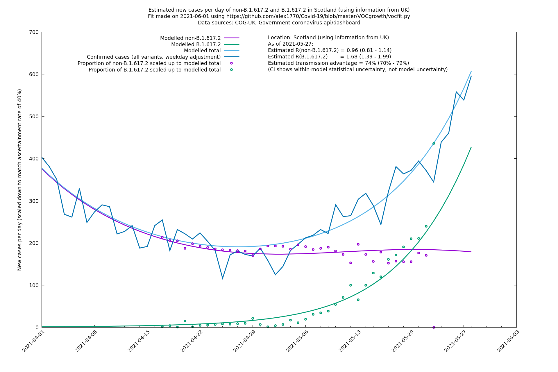
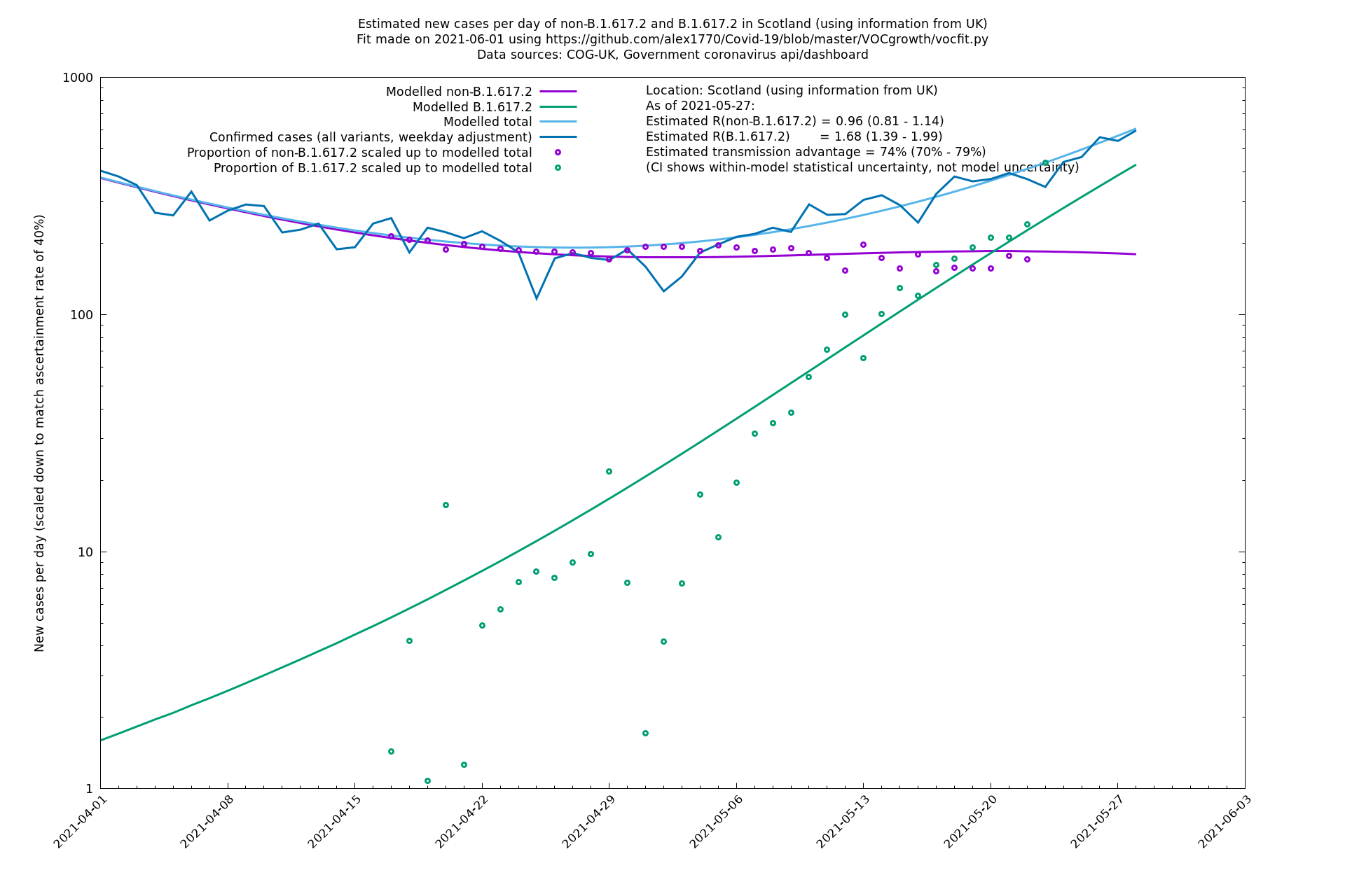
| Scotland | UK | COG-UK | 74% (70% - 79%) | 0.96 (0.81 - 1.14) | 1.68 (1.39 - 1.99) |
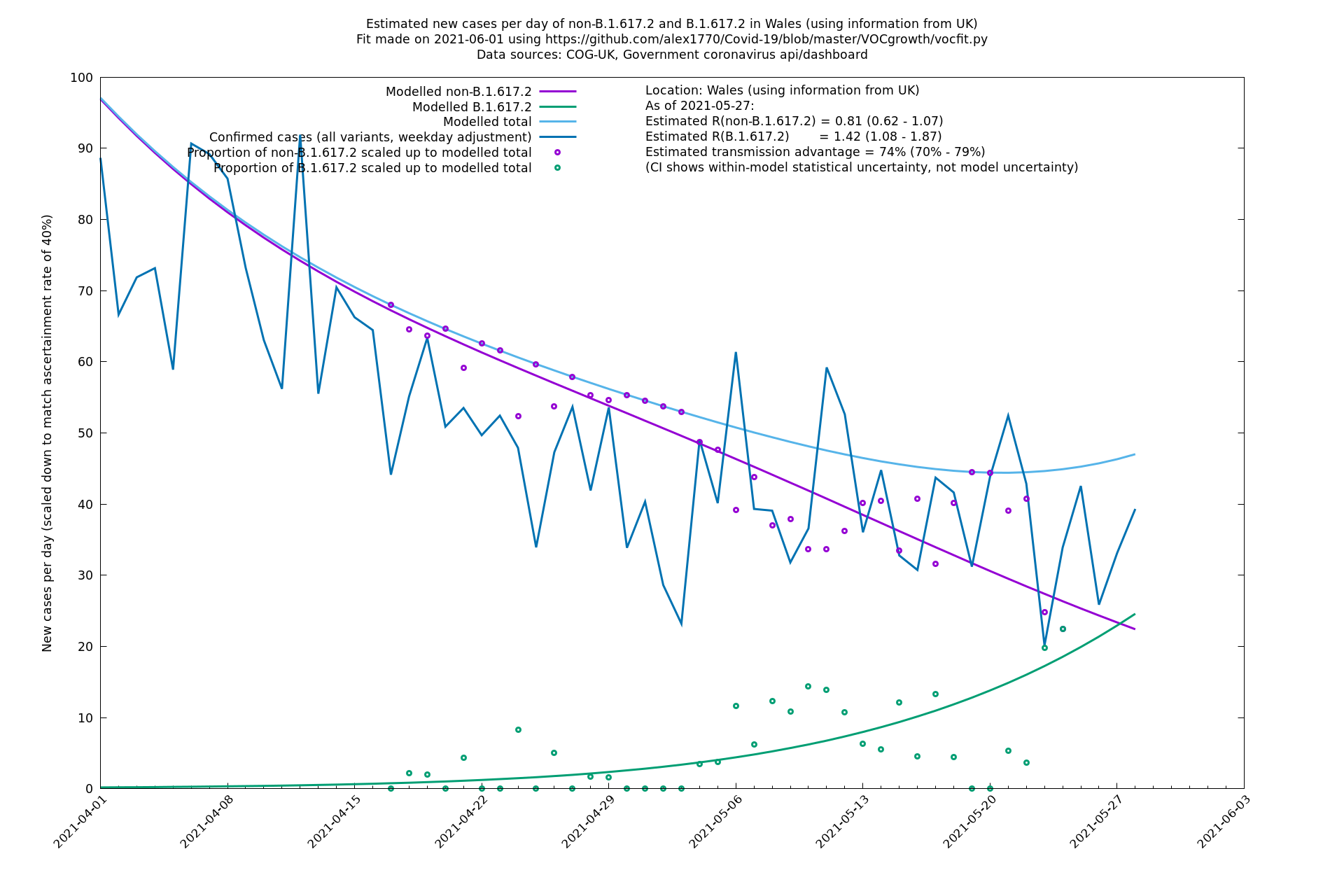
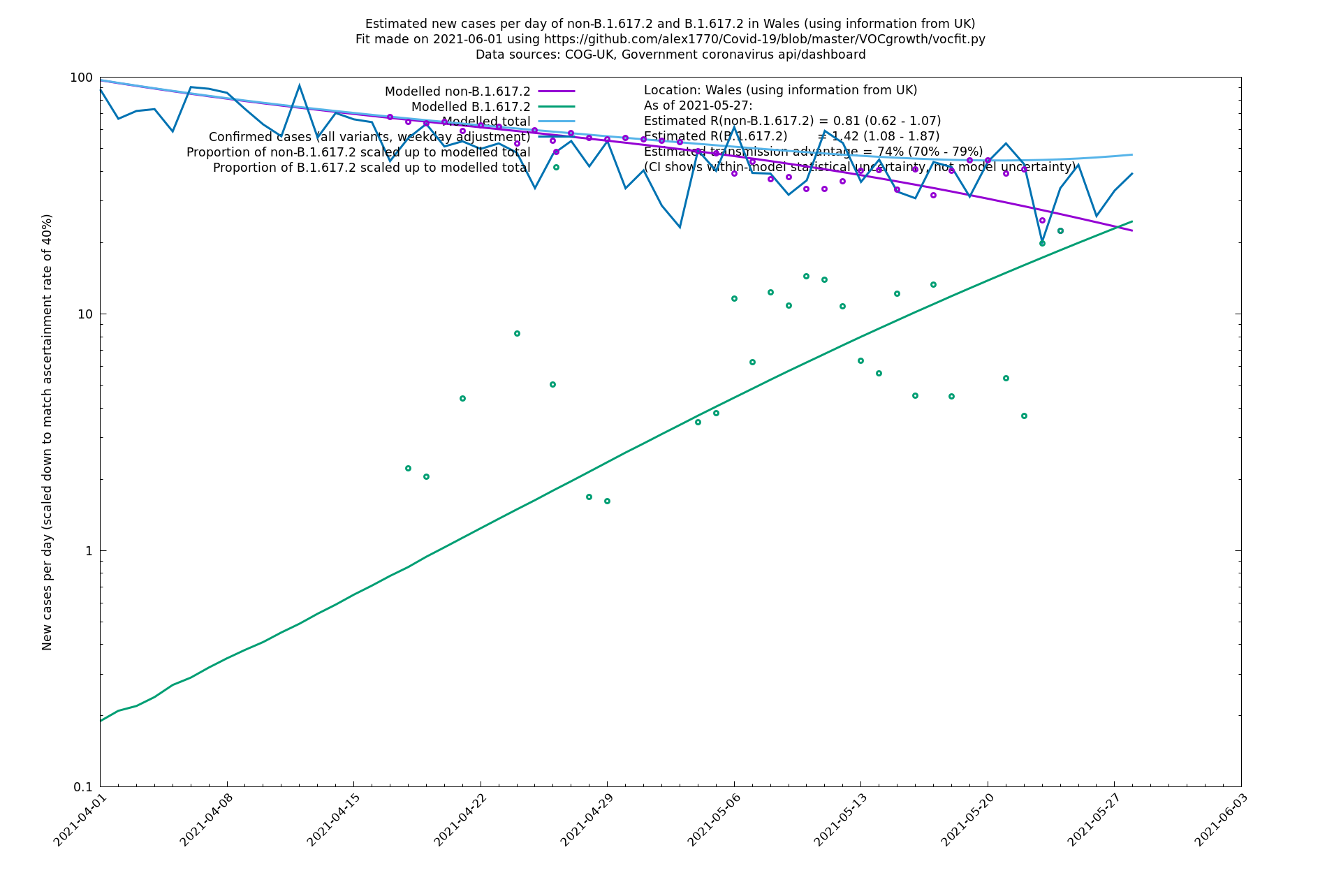
| Wales | UK | COG-UK | 74% (70% - 79%) | 0.81 (0.62 - 1.07) | 1.42 (1.08 - 1.87) |
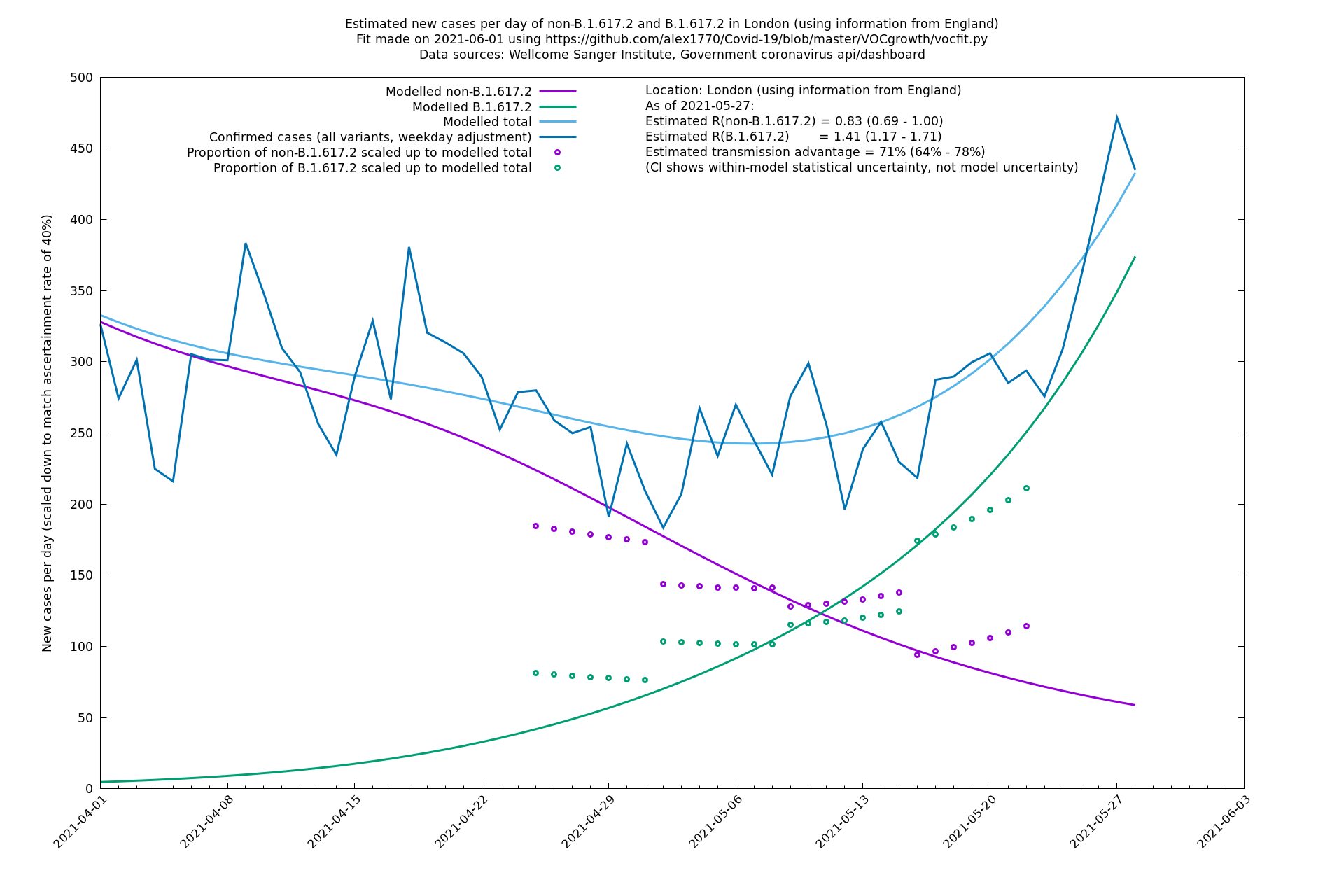
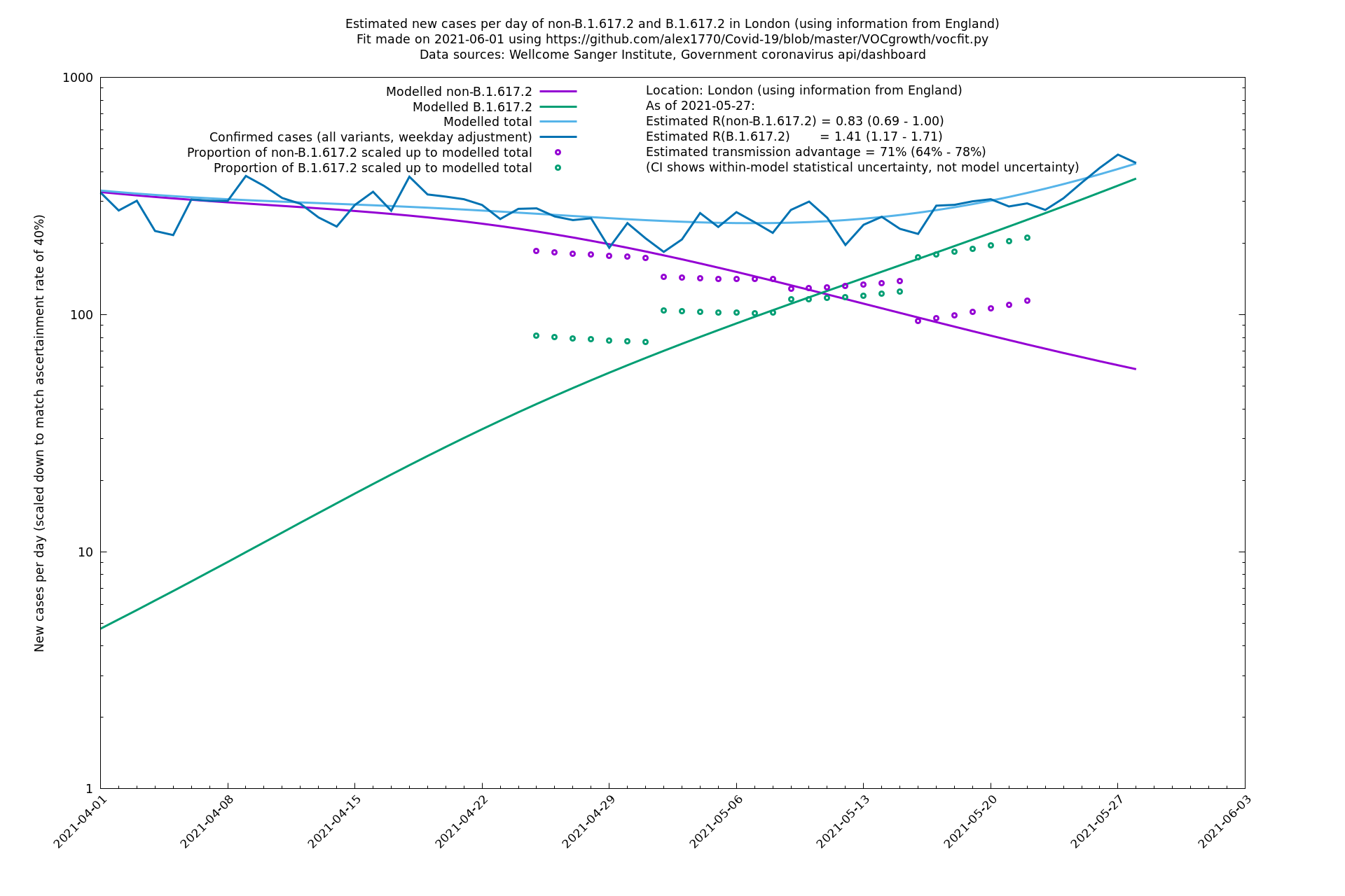
| London | London LTLAs | Sanger | 44% (24% - 68%) | 0.92 | 1.29 (1.12 - 1.57) |
| London | England | Sanger | 71% (64% - 78%) | 0.83 (0.69 - 1.00) | 1.41 (1.17 - 1.71) |
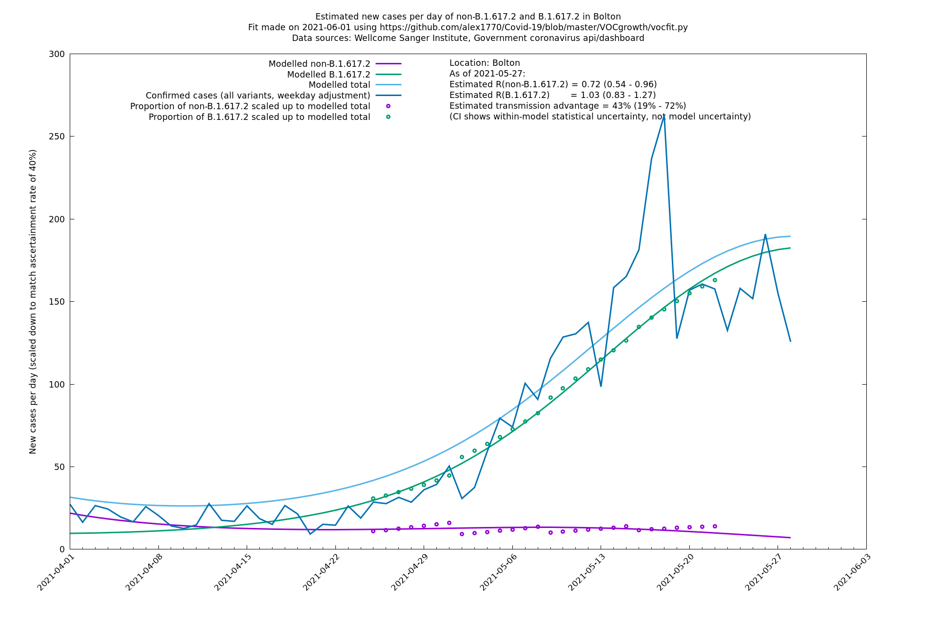
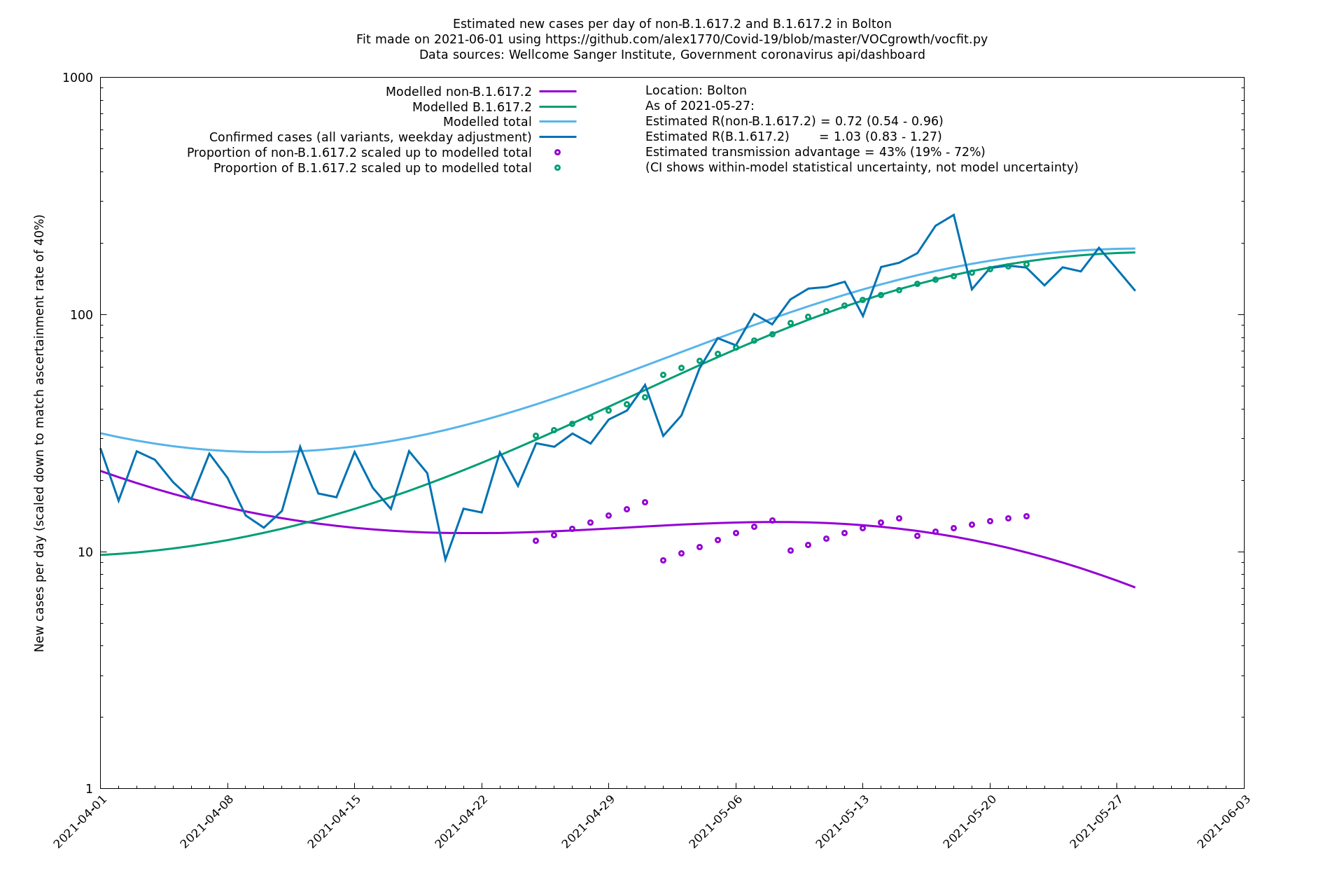
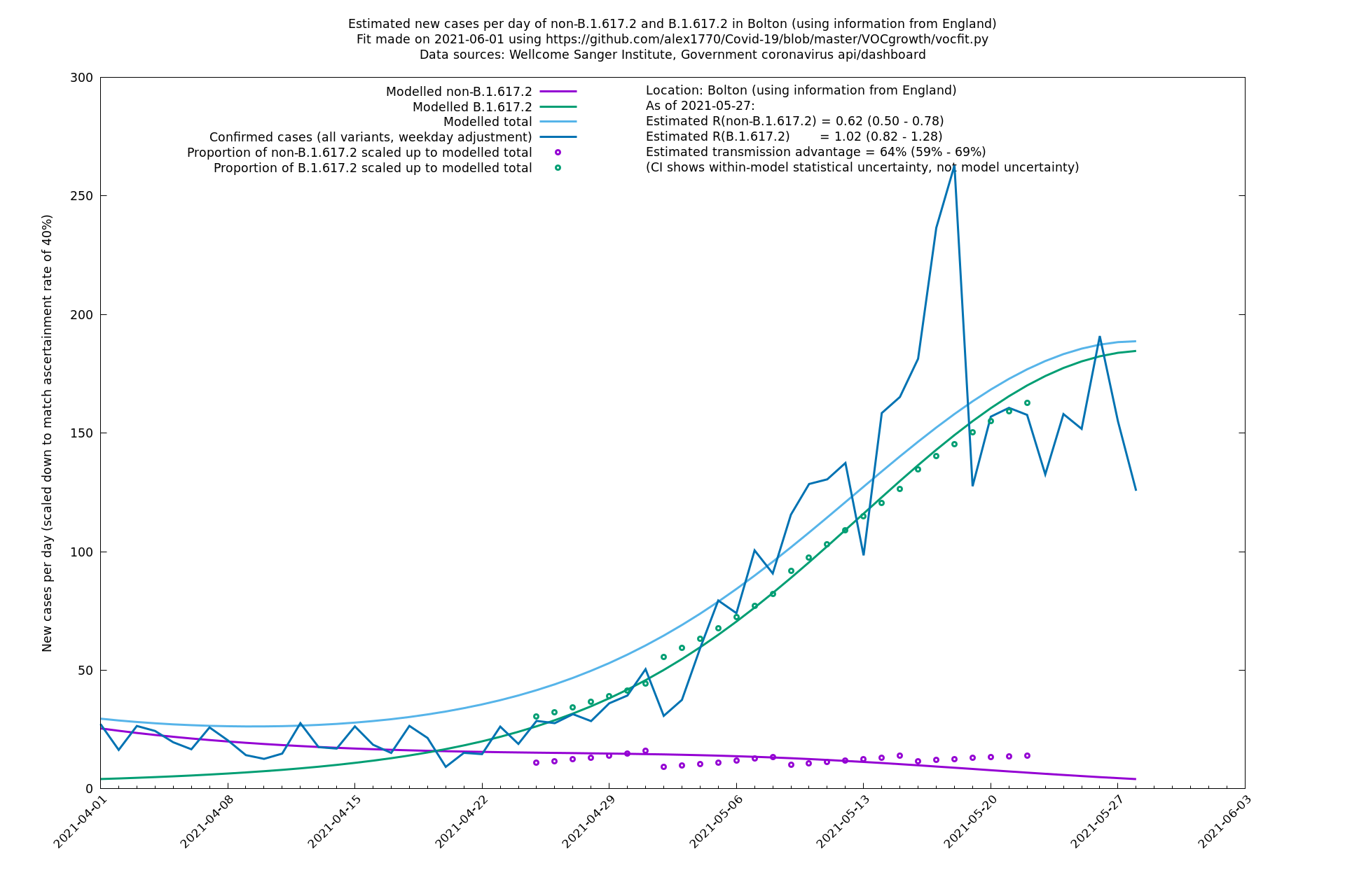
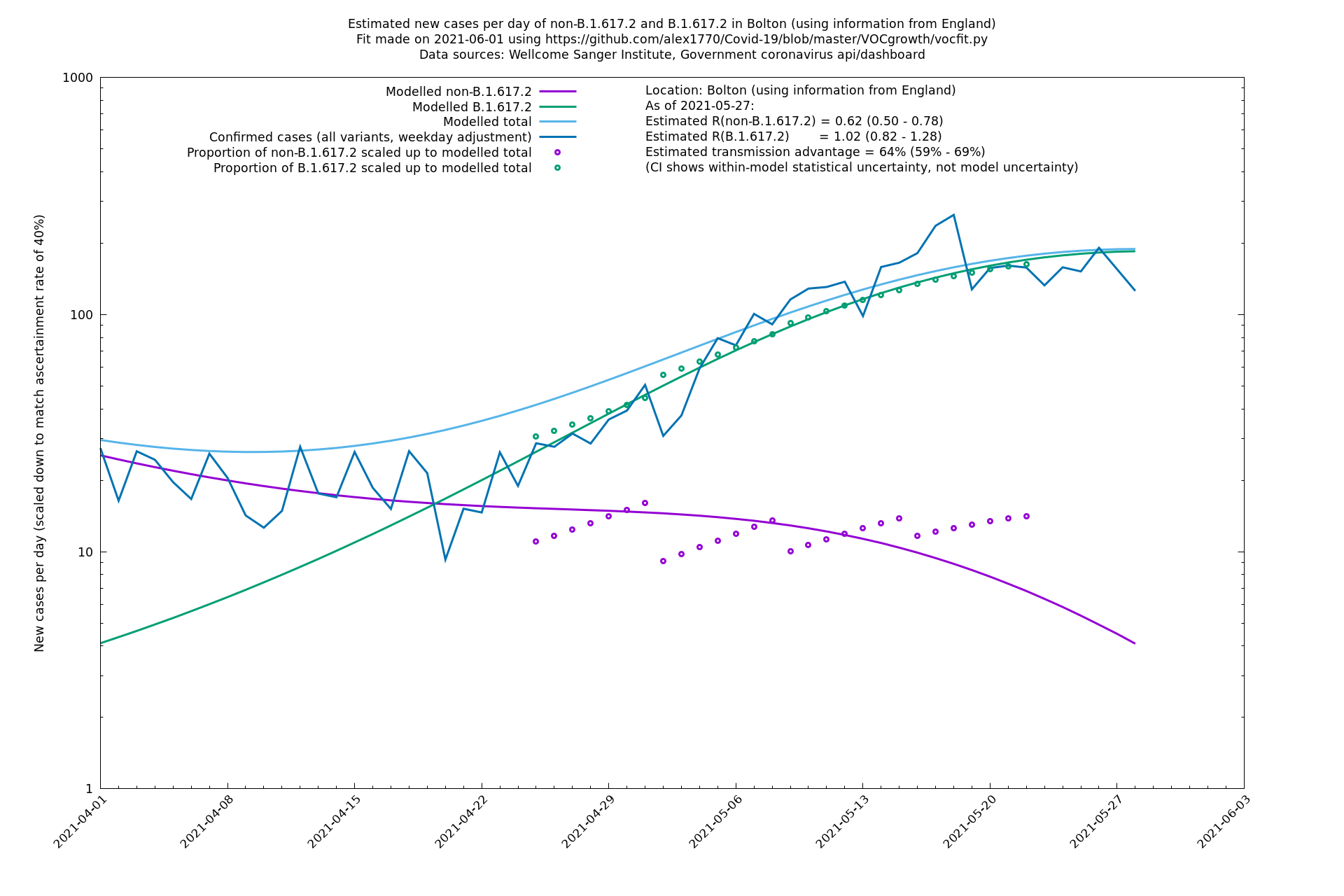
| Bolton | England | Sanger | 72% (62% - 83%) | 0.59 (0.47 - 0.75) | 1.02 (0.81 - 1.30) |
The numbers are high overall, with an R number of around 1.5 for B.1.617.2 in most of the UK, though it is striking that Bolton seems to have controlled the outbreak.
NB: the confidence intervals in the above table underestimate the uncertainty, because the model relies on assumptions which may not be completely correct.
NB2: The above estimates are not independent of each other because, in this mode, the model is using information from around the country to inform the more local estimates. We can illustrate this by the following two different runs that estimate parameters for the regions of England.
In the following table, the transmission advantages are conditioned to be equal for all regions. This is a good mode to use if you already believe that the transmission advantages are necessarily the same around the country, since it pools all the data and reduces statistical fluctuation.
| Location | Using information from | Data source (Sanger to w/e 2021-05-15) | Estimated transmission advantage | Estimated $$R_{B.1.1.7}$$ on 2021-05-29 | Estimated $$R_{B.1.617.2}$$ on 2021-05-29 |
|---|---|---|---|---|---|
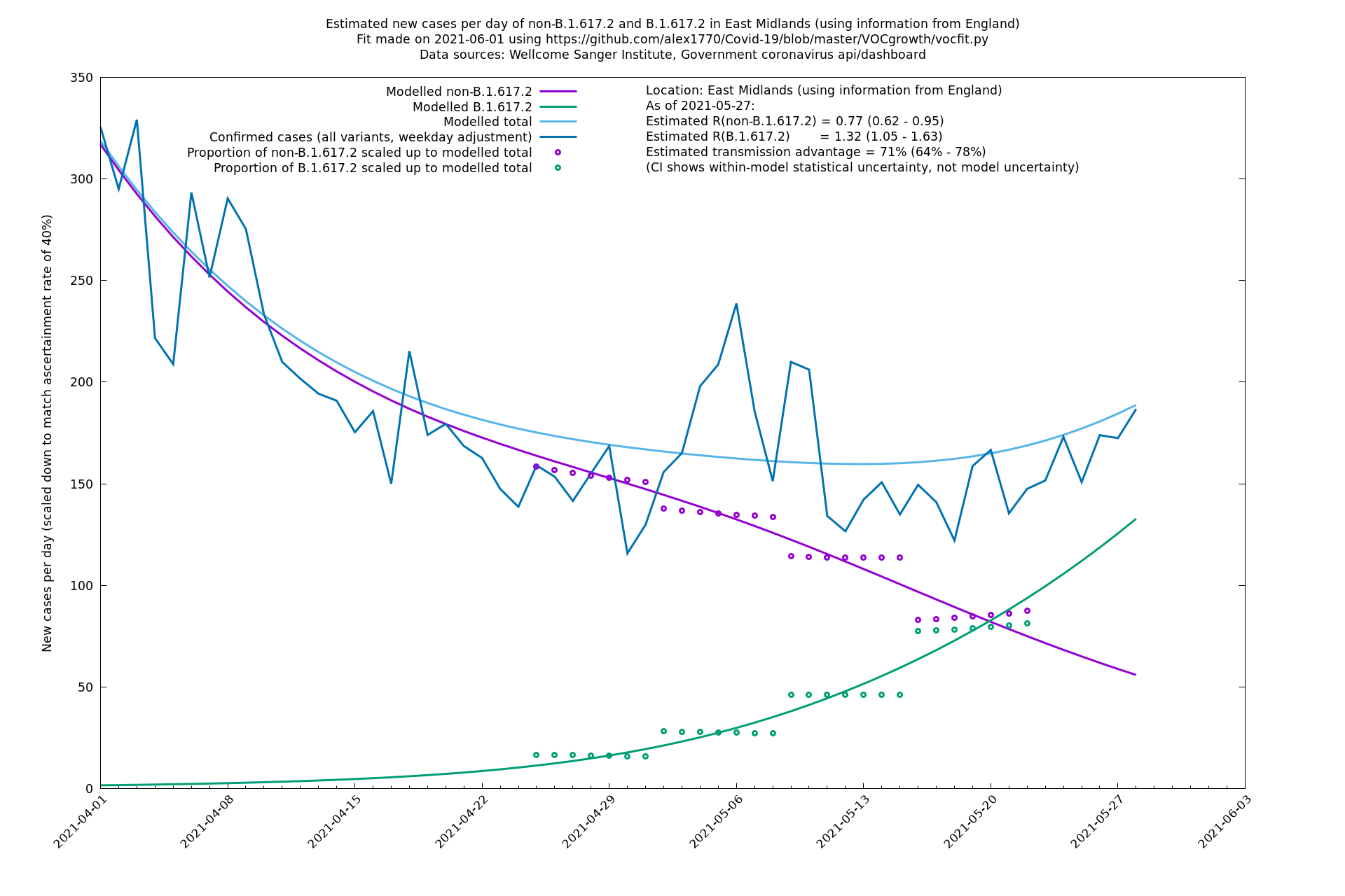
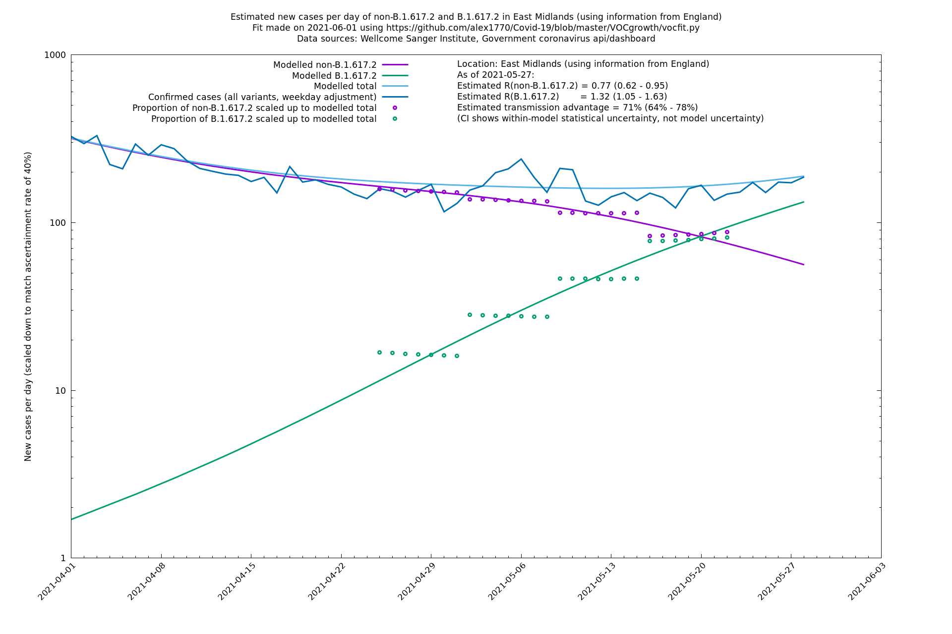
| East Midlands | England | Sanger | 74% (66% - 82%) | 0.74 (0.60 - 0.92) | 1.29 (1.04 - 1.62) |
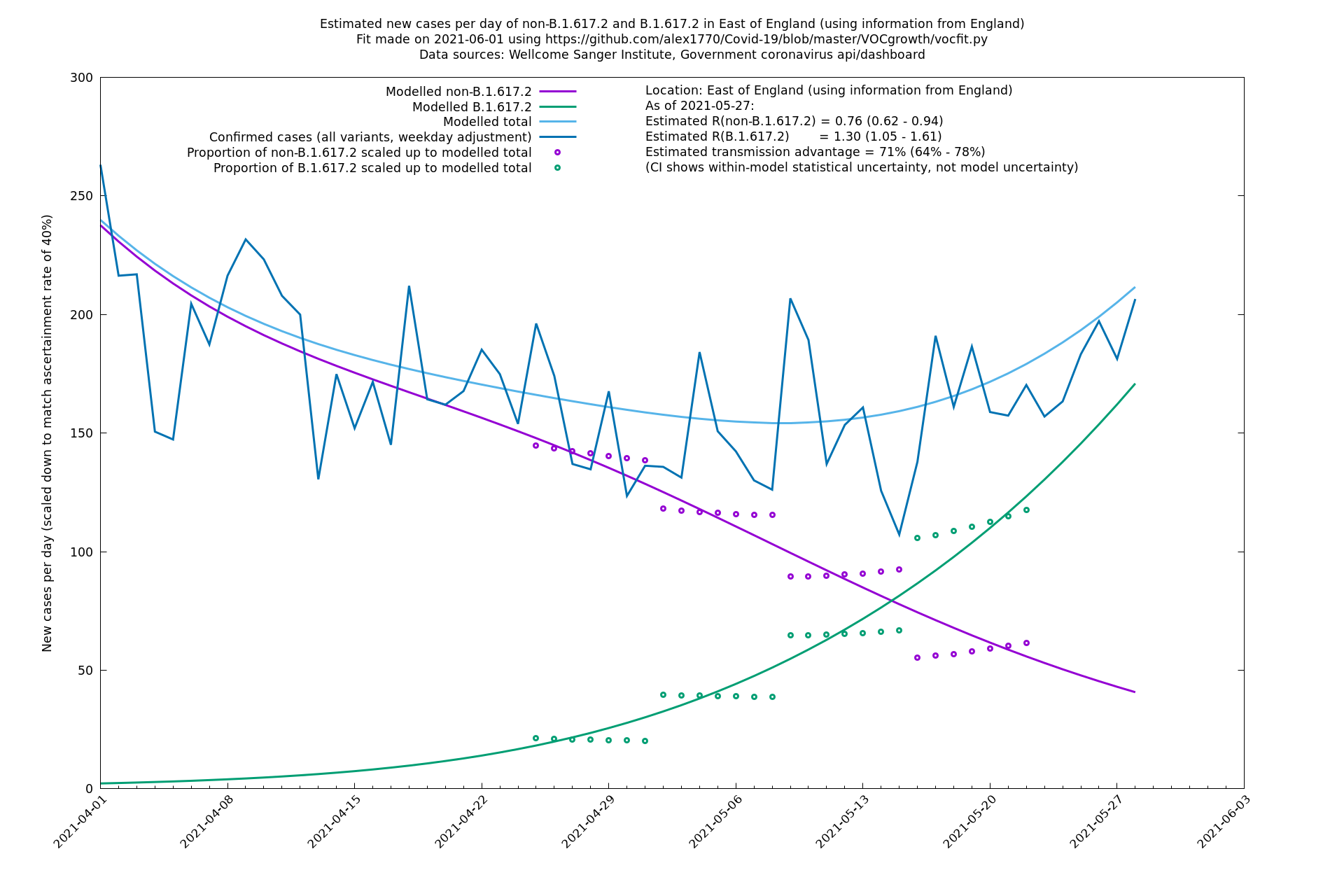
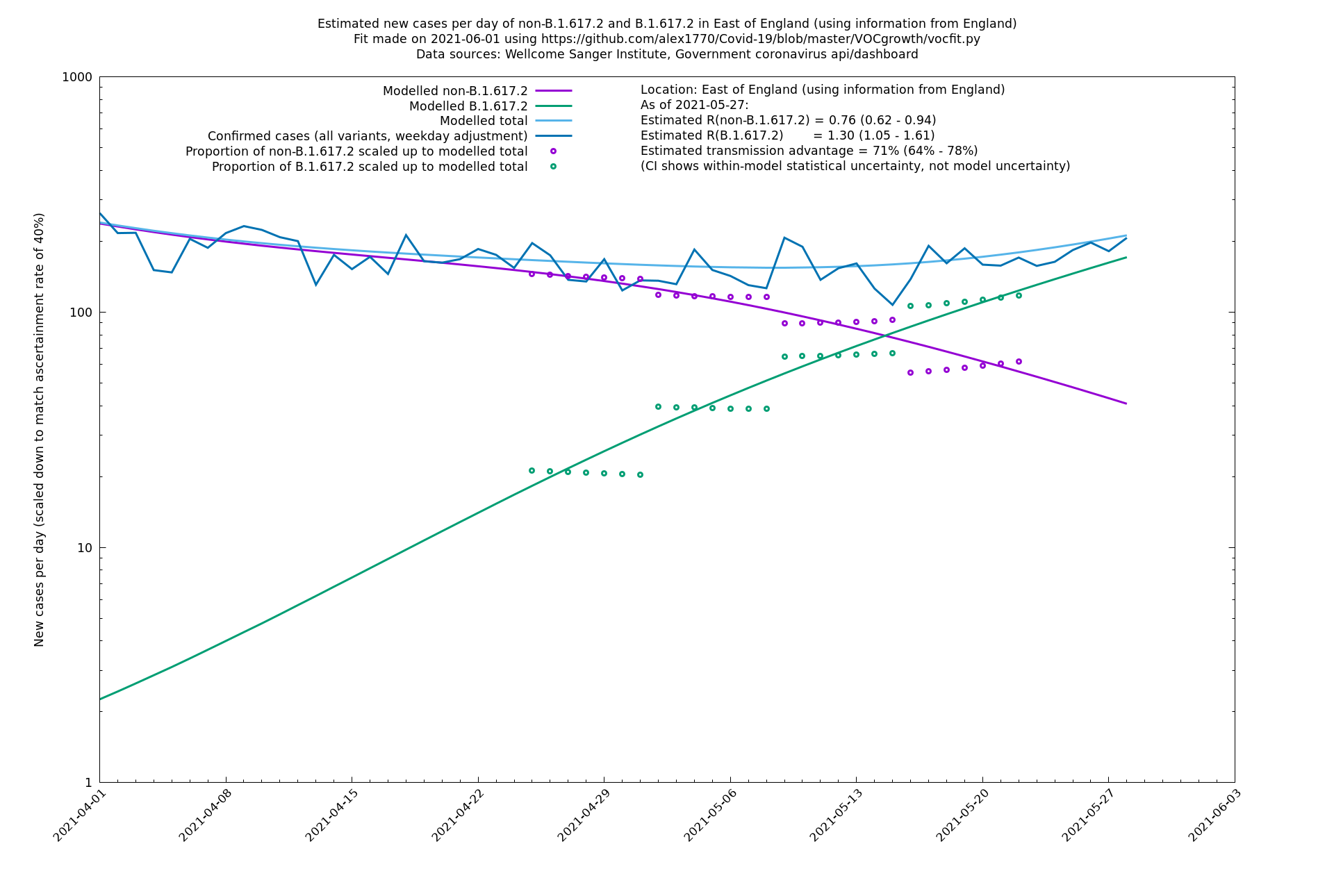
| East of England | England | Sanger | 74% (66% - 82%) | 0.71 (0.57 - 0.88) | 1.24 (0.98 - 1.54) |
| London | England | Sanger | 74% (66% - 82%) | 0.80 (0.66 - 0.95) | 1.39 (1.15 - 1.68) |
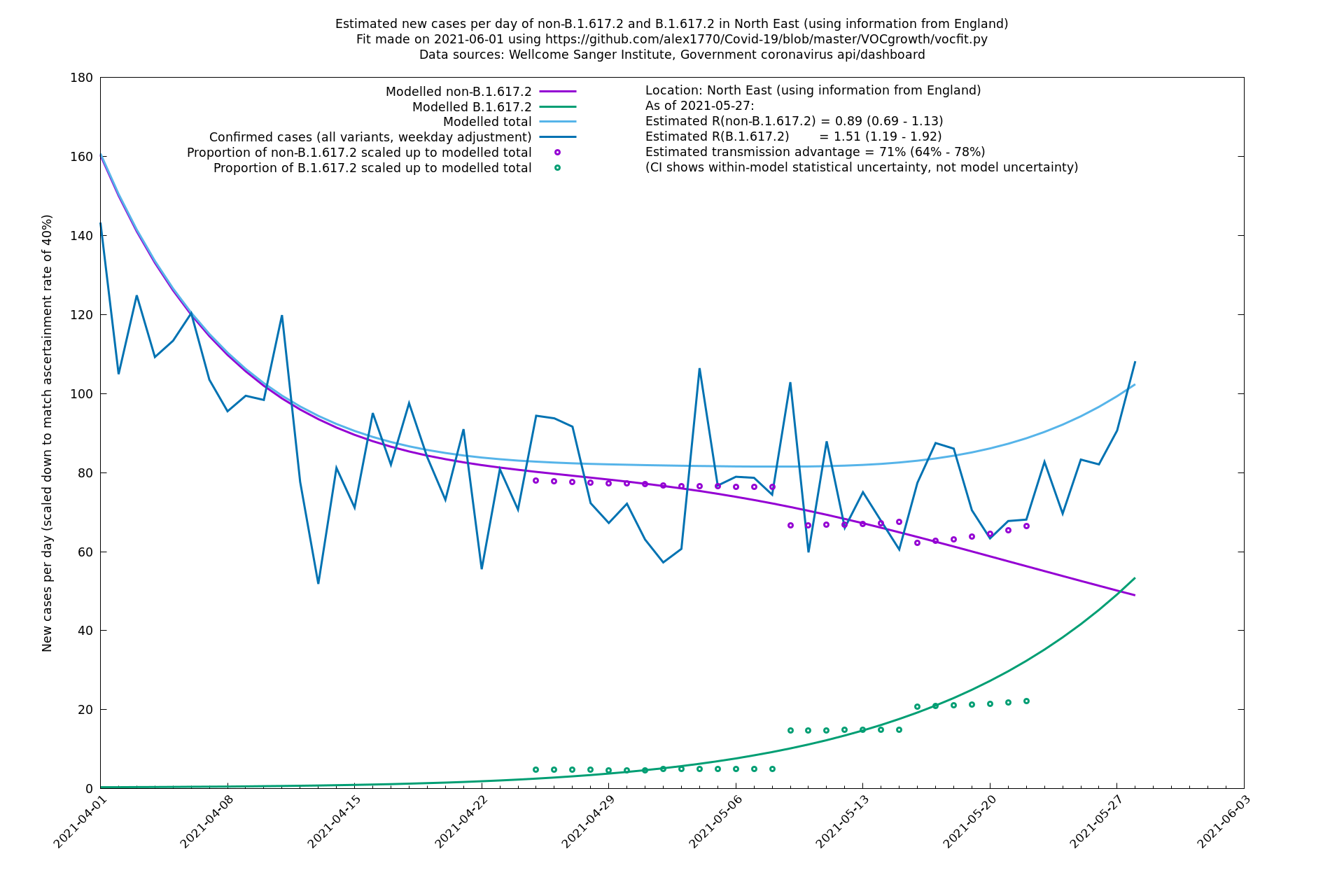
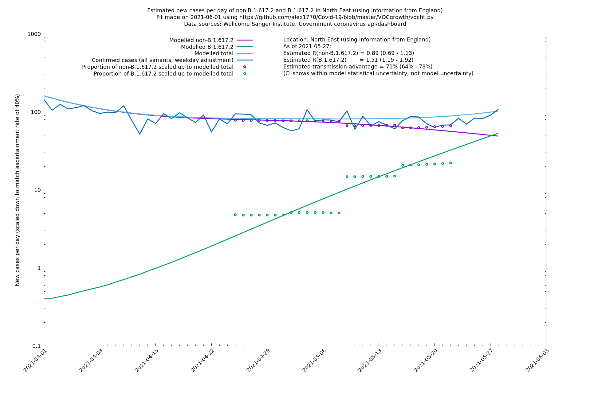
| North East | England | Sanger | 74% (66% - 82%) | 0.89 (0.68 - 1.17) | 1.54 (1.17 - 2.03) |
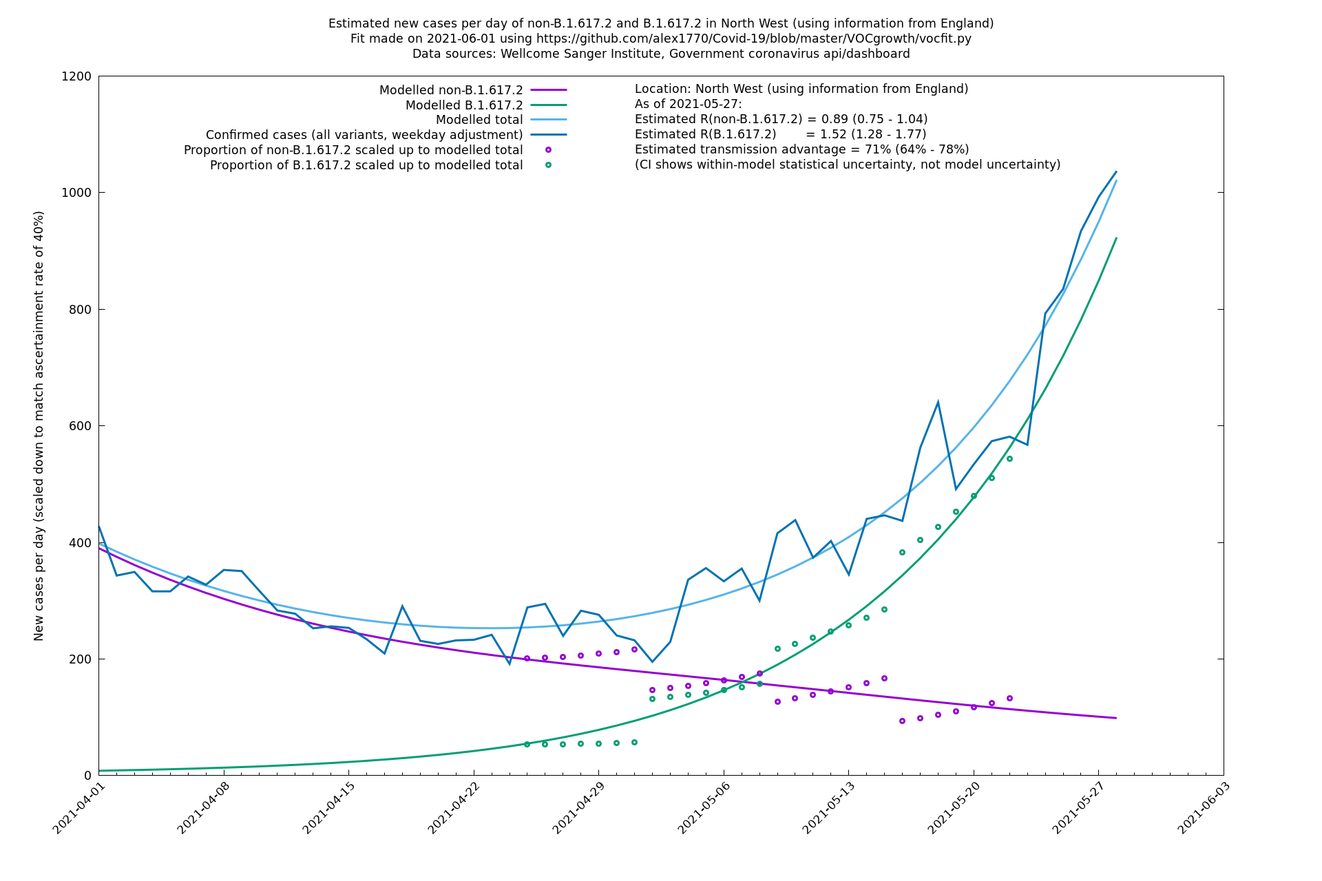
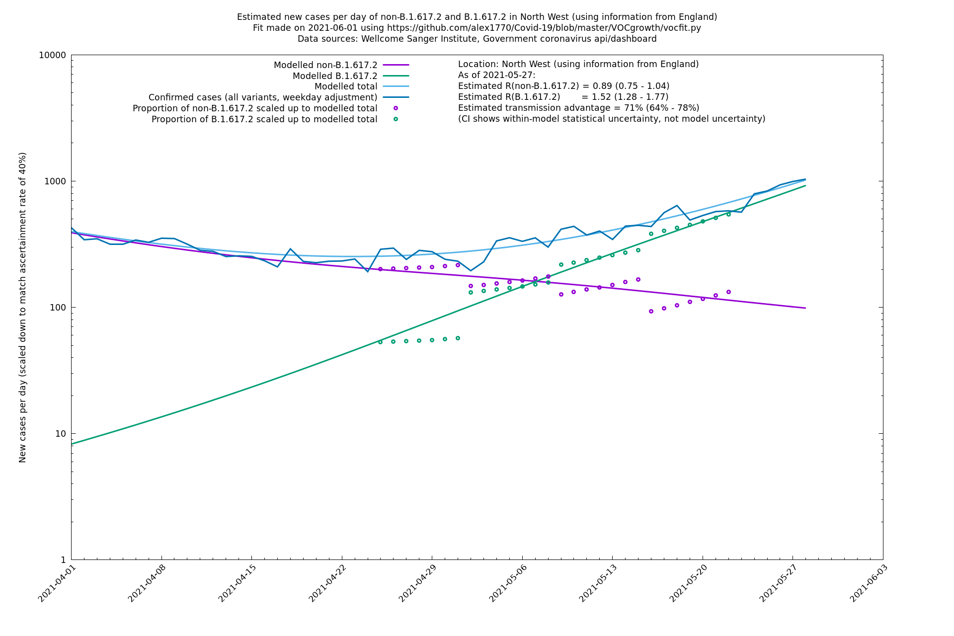
| North West | England | Sanger | 74% (66% - 82%) | 0.82 (0.70 - 0.95) | 1.43 (1.22 - 1.67) |
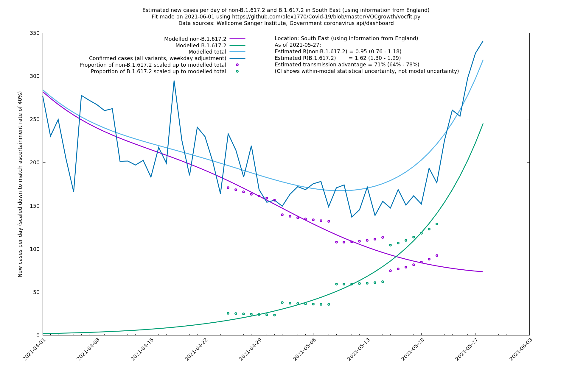
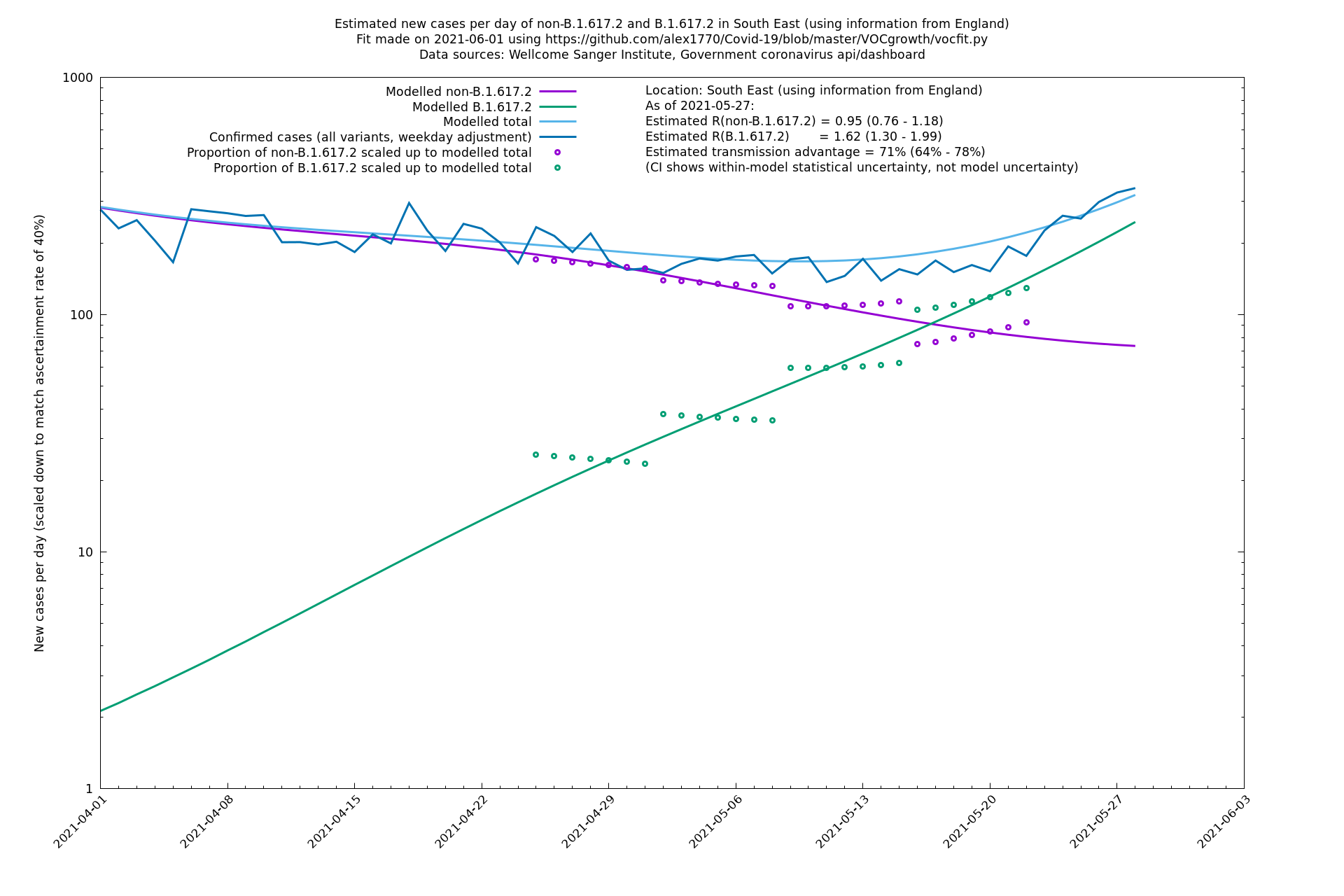
| South East | England | Sanger | 74% (66% - 82%) | 0.94 (0.76 - 1.15) | 1.63 (1.32 - 2.01) |
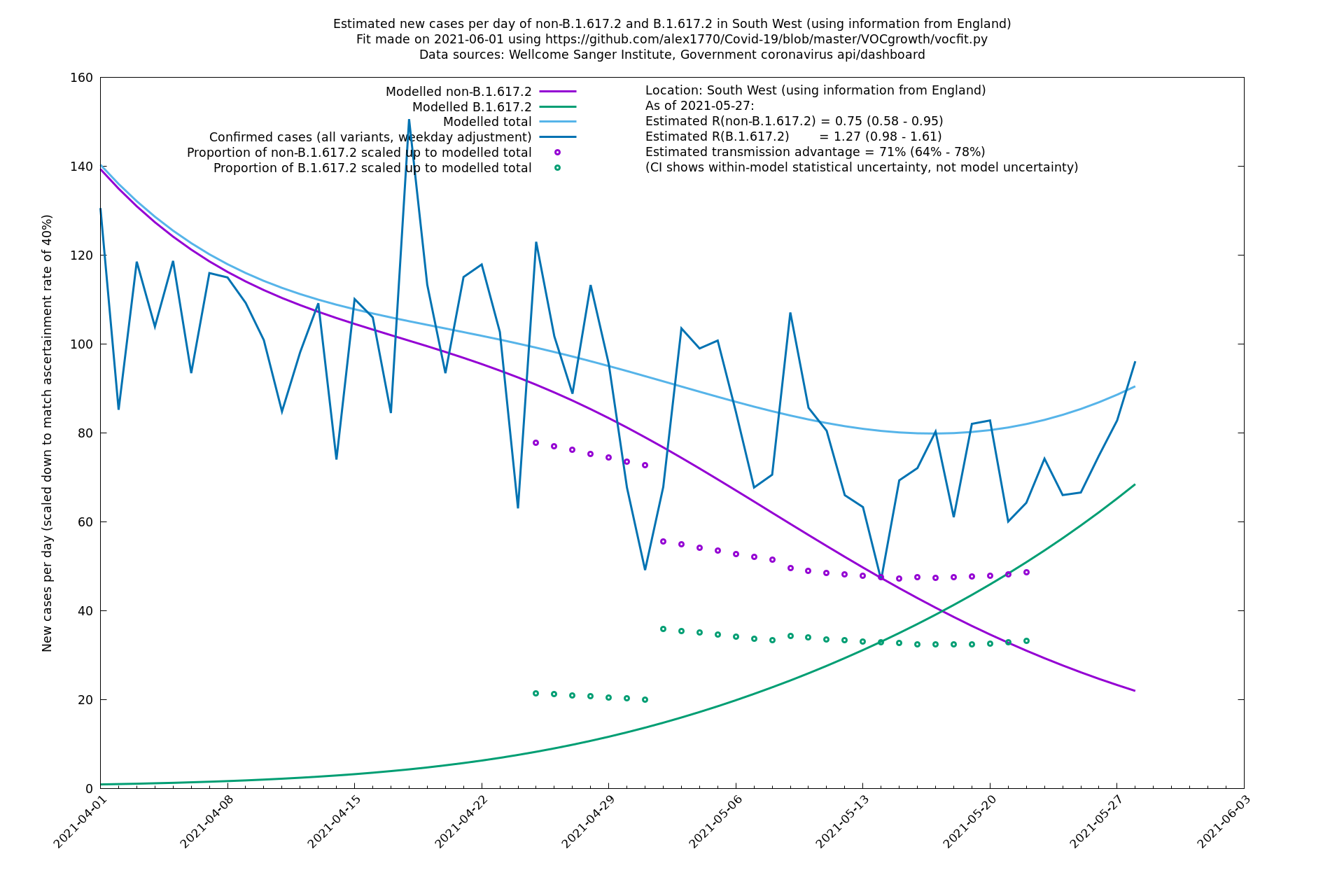
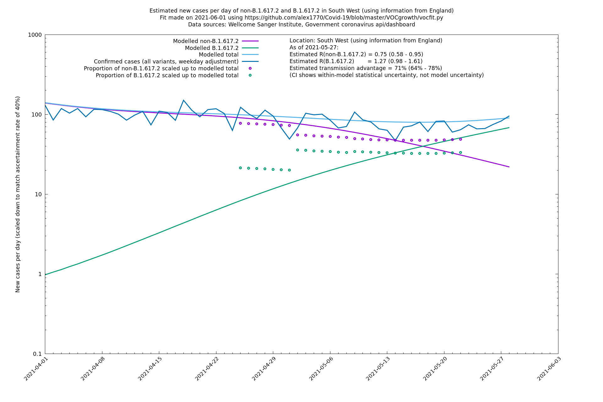
| South West | England | Sanger | 74% (66% - 82%) | 0.74 (0.57 - 0.96) | 1.28 (0.99 - 1.68) |
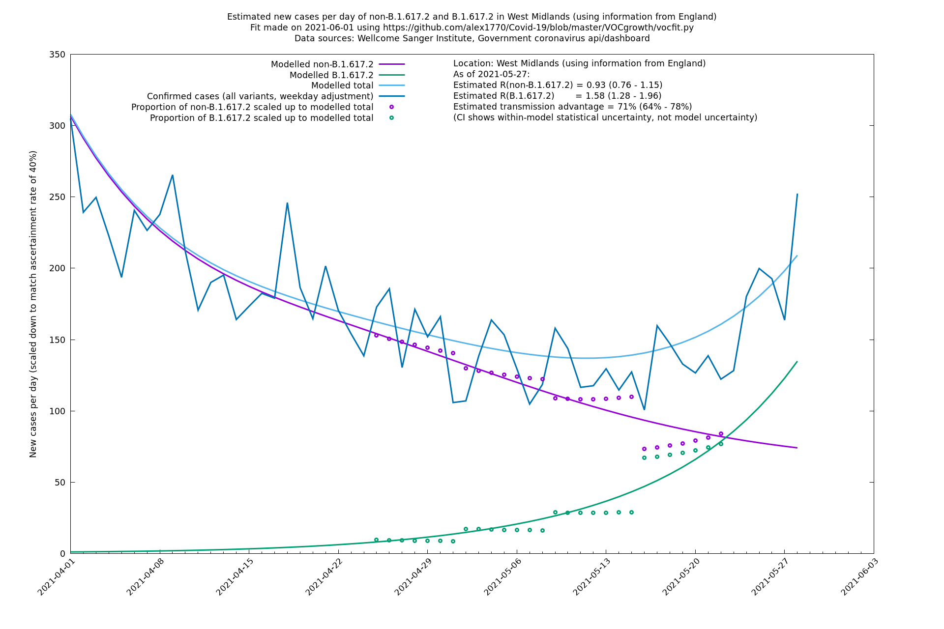
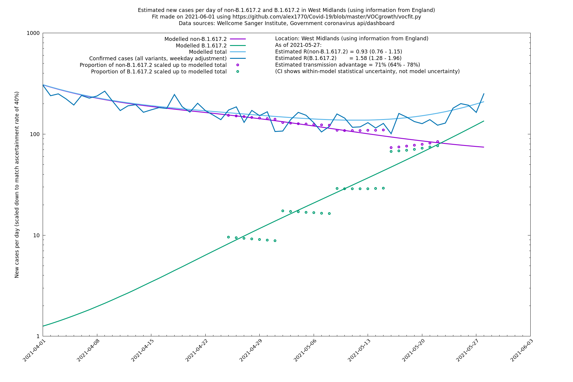
| West Midlands | England | Sanger | 74% (66% - 82%) | 0.92 (0.74 - 1.14) | 1.59 (1.28 - 2.01) |
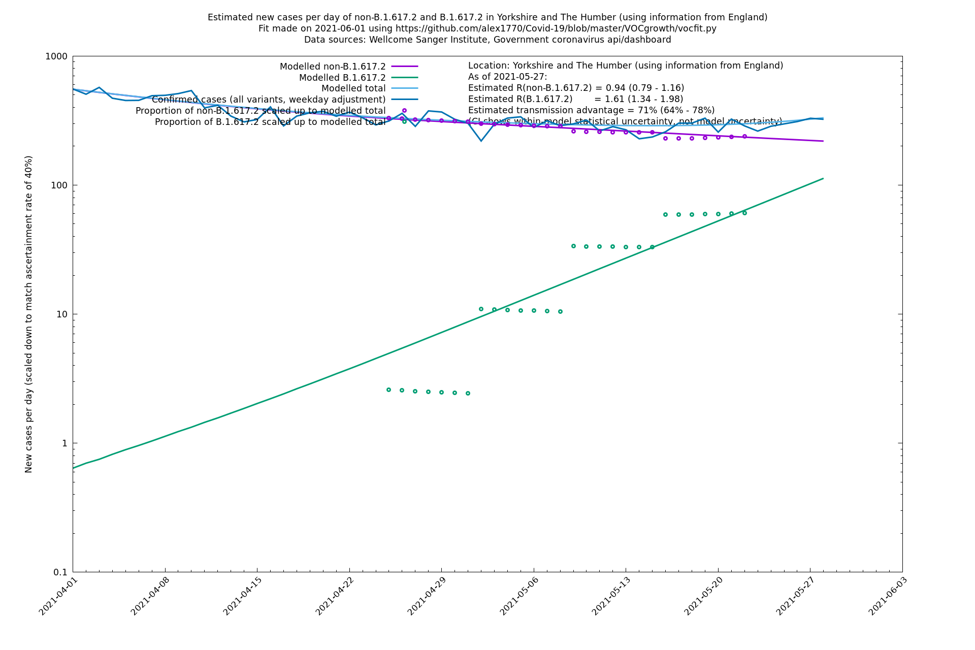
| Yorkshire and The Humber | England | Sanger | 74% (66% - 82%) | 0.93 (0.76 - 1.14) | 1.62 (1.32 - 1.99) |
On the other hand, in the next table all regions are run separately. This is a good mode to use if you want to test the hypothesis that the transmission advantage is the same around the country. The confidence intervals are very wide in several regions because they haven't had many B.1.617.2 infections (as of early/mid May when the Sanger dataset was updated), but it is still notable that London seems to have lower transmission advantage than the average.
| Location | Using information from | Data source (Sanger to w/e 2021-05-15) | Estimated transmission advantage | Estimated $$R_{B.1.1.7}$$ on 2021-05-29 | Estimated $$R_{B.1.617.2}$$ on 2021-05-29 |
|---|---|---|---|---|---|
| East Midlands | - | Sanger | 67% (48% - 88%) | 0.77 (0.60 - 0.99) | 1.29 (1.03 - 1.61) |
| East of England | - | Sanger | 81% (60% - 104%) | 0.68 (0.53 - 0.88) | 1.24 (0.99 - 1.54) |
| London | - | Sanger | 40% (24% - 58%) | 1.00 (0.81 - 1.25) | 1.41 (1.17 - 1.69) |
| North East | - | Sanger | 51% (-2% - 133%) | 0.97 (0.68 - 1.37) | 1.47 (1.06 - 2.02) |
| North West | - | Sanger | 84% (71% - 97%) | 0.77 (0.65 - 0.91) | 1.41 (1.21 - 1.65) |
| South East | - | Sanger | 76% (49% - 108%) | 0.93 (0.71 - 1.21) | 1.63 (1.33 - 1.99) |
| South West | - | Sanger | 20% (-11% - 63%) | 0.93 (0.68 - 1.25) | 1.11 (0.83 - 1.49) |
| West Midlands | - | Sanger | 92% (64% - 124%) | 0.84 (0.65 - 1.08) | 1.62 (1.30 - 2.00) |
| Yorkshire and The Humber | - | Sanger | 99% (55% - 155%) | 0.86 (0.65 - 1.12) | 1.70 (1.37 - 2.12) |
Model details
We treat the generation time for both variants as a constant (5 days). This implies that the ratio of R-numbers being a constant is the same as the difference in growth rates being a constant. In general these two conditions are slightly different things if the generation time is not constant, but it is likely to be a good approximation here. If the generation time were distributed as $$\Gamma(7.886, 1.633)$$ (shape, rate notation) as suggested by the meta-analysis of Challen et al, then the growth rate and reproduction number would, using the standard formula, be related by $$R=(1+g/1.633)^{7.886}$$, which means for two different variants, $$g'-g=1.633(T^{0.127}-1)R^{0.127}$$ where $$T=R'/R$$. For a given $$T$$, $$g'-g$$ can only vary by a factor of $$R^{0.127}$$ and since we believe the reproduction number of B.1.1.7 is mostly stable at around $$0.7-1.0$$, the variation in $$R^{0.127}$$ is only about 4-5% which means for practical purposes we can probably take $$g'-g$$ as fixed.
The log likelihood, $$L(A,h)$$, for each area is given by this model:
Constants and known variables (observed data): \[ \begin{equation*} \begin{split} n_i &= \text{number of confirmed cases on day } i \text{ (counts are slightly adjusted to compensate for weekday effect)}\\ p &= \text{case ascertainment rate (proportion of cases that are discovered by PCR test)}\\ g_{-1}(\rho),v_{-1}(\rho)&=\text{empirical growth rate (and its variance) in the two weeks up to 2021-04-10 as a function of region, }\rho\\ r_j, s_j &= \text{Counts of non-B.1.617.2, B.1.617.2 respectively in the } j^{\text{th}} \text{ week}\\ I_j &= \text{set of days (a day for COG-UK; a week for Sanger) corresponding to the above VOC counts } r_j, s_j\\ f_1 &= \text{a constant used to allow for overdispersion of case counts}\\ f_2 &= \text{a constant used to allow for overdispersion of variant counts}\\ g_\text{lengthscale}&= \text{a constant which scales the growth parameters}\\ g_\text{timescale}&= \text{a constant setting the timescale over which the growth rate is allowed to vary} \end{split} \end{equation*} \]
Unknown/latent variables/parameters: \[ \begin{equation*} \begin{split} h&=\text{daily growth advantage of B.1.617.2 over other variants}\\ X_n&=\text{Fourier coefficients controlling the growth of non-B.1.617.2}\\ A_0&=\text{initial count of non-B.1.617.2}\\ B_0&=\text{initial count of B.1.617.2}\\ \end{split} \end{equation*} \]
Likelihood/distributions (and definitions of intermediate terms), where $$i=0,\ldots,D-1$$ or $$i=0,\ldots,D$$, and $$D=$$(number of days), $$N=D+2g_\text{timescale}$$: \[ \begin{equation*} \begin{split} A_{i+1}&=e^{g_i}A_i\\ B_{i+1}&=e^{g_i+h}B_i\\ \widetilde{A_j}&=\sum_{i\in I_j}A_i\\ \widetilde{B_j}&=\sum_{i\in I_j}B_i\\ n_i &\sim \text{Negative Binomial}(\mu=p(A_i+B_i),\text{variance=}\mu(1+f_1^{-1}))\\ r_j,s_j &\sim \text{Beta Binomial}(r_j+s_j,f_2\widetilde{A_j},f_2\widetilde{B_j})\\ g_0&\sim N(g_{-1},v_{-1})\\ X_n&\sim N(0,1)\\ g_i&=g_0+g_\text{lengthscale}\sqrt{N}\left(\frac{i}{N}X_0+\frac{\sqrt2}{\pi}\sum_{n=1}^{[3N/g_\text{timescale}]}e^{-(ng_\text{timescale}/N)^2/2}\frac{\sin(n\pi i/N)}{n}X_n\right)\\ h&\sim N(0,\tau^2)\\ \end{split} \end{equation*} \]
A bit about the motivation for these choices: growth rates (or reproduction numbers) for each variant can change over time, so it is desirable to allow for some time-variation in these. Keeping the growth rate of the two variants separated by a universal constant ($$h$$) seems like a plausible assumption which allows us to make decent predictions. The formula for $$g_i$$ is a kind of low-pass filtered Brownian motion (the variance of the Fourier coefficients being in a certain proportion). This parametrizes a nice space of smooth functions that may possibly work better than, for example, splines because it is low dimensional and hopefully characterises the kind of "wiggles" that are likely to occur. The parameter space being of relatively low dimension makes it fast and robust to analyse. We choose $$N>D$$ to remove boundary/periodicity effects since the space of parametrized functions is periodic in $$N$$ plus a drift term. The beta-binomial is used as an "overdispersed" binomial distribution. We don't try to model $$r_j+s_j$$, only $$r_j, s_j$$ conditioned on $$r_j+s_j$$. The reason for this is that we don't want/need to get into predicting what proportion of cases are sequenced, because it's volatile and not relevant to inferring the true proportion of variants, assuming there is no bias relating overall number of variant counts to the proportion of the new variant. Doing it this way has the benefit that we can use recent, incomplete, variant counts alongside older, complete ones. [In fact we use the negative binomial and beta-binomial for training, but variance-scaled-Poisson and variance-scaled-Binomial with corresponding parameters for runs. Writeup to be completed later.]
The log likelihood, including the prior for the parameters (and omitting some constant terms) is then \[ \sum_i \left(\log\left(\frac{\Gamma(n_i+f_1\mu_i)}{\Gamma(f_1\mu_i)\Gamma(n_i+1)}\right)+f_1\mu_i\log\left(\frac{f_1}{1+f_1}\right)+n_i\log\left(\frac{1}{1+f_1}\right)\right)\\ +\sum_j \log\left(\binom{r_j+s_j}{r_j}\frac{B(f_2\widetilde{A_j}+r_j,f_2\widetilde{B_j}+s_j)}{B(f_2\widetilde{A_j},f_2\widetilde{B_j})}\right)\\ -\frac{(g_0-g_{-1})^2}{2v_{-1}}-\frac12\sum_n X_n^2-\frac{h^2}{2\tau^2}, \text{ where}\\ \mu_i=p(A_i+B_i), A_r=A_0e^{\sum_{i<r}g_i}, B_r=B_0e^{rh+\sum_{i<r}g_i}, \text{ and}\\ g_i=g_0+g_\text{lengthscale}\sqrt{N}\left(\frac{i}{N}X_0+\frac{\sqrt2}{\pi}\sum_{n=1}^{[3N/g_\text{timescale}]}e^{-(ng_\text{timescale}/N)^2/2}\frac{\sin(n\pi i/N)}{n}X_n\right) \] and can be maximised over $$h$$, $$A_0$$, $$B_0$$, $$g_0$$ and $$X_n$$.
After the MLE has been found, the log likelihood can be expanded about the maximum and the quadratic approximation yields a Gaussian which can be integrated (Laplace approximation), giving a good approximation of the integral of the likelihood over the parameter space of $$h$$, $$A_0$$, $$B_0$$, $$g_0$$ and $$X_n$$. This gives the proper normalisation which allows one to optimise over $$f_1$$, $$f_2$$, $$g_\text{timescale}$$, $$g_\text{lengthscale}$$. Trained on the UK with COG-UK data, we're currently using $$f_1=0.050$$, $$f_2=0.075$$, $$g_\text{timescale}=25$$, $$g_\text{lengthscale}=0.01$$. The other constants don't make much difference to the estimates or confidence intervals. With further work, the four constants could be incorporated as dynamic parameters which would allow for fluctuation in these "constants", and also allow for different values of these in different regions.
Confidence intervals for $$h$$, the growth rate difference between the two variants, are easy to obtain because $$h$$ is one of the parameters, so as mentioned previously it is just a matter of calculating $$(-L''(A,h^*))^{-1/2}$$. To calculate confidence intervals for other features, such as $$R_{B.1.617.2}$$, the parameters are treated as normal distributions centred on the MLE, with covariance matrix given by the inverse Hessian of the log likelihood. This is an alternative to using something like Markov Chain Monte Carlo.
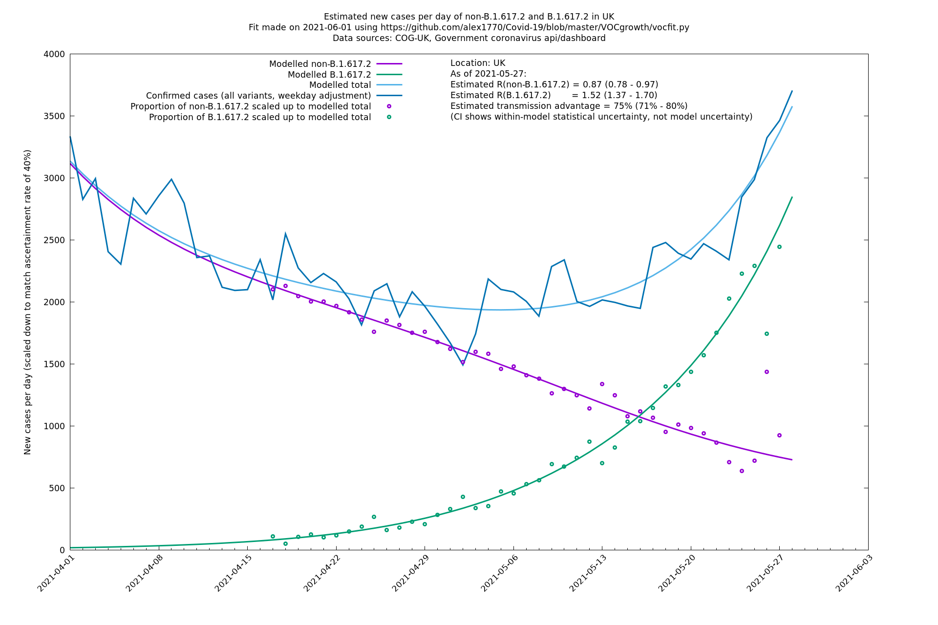
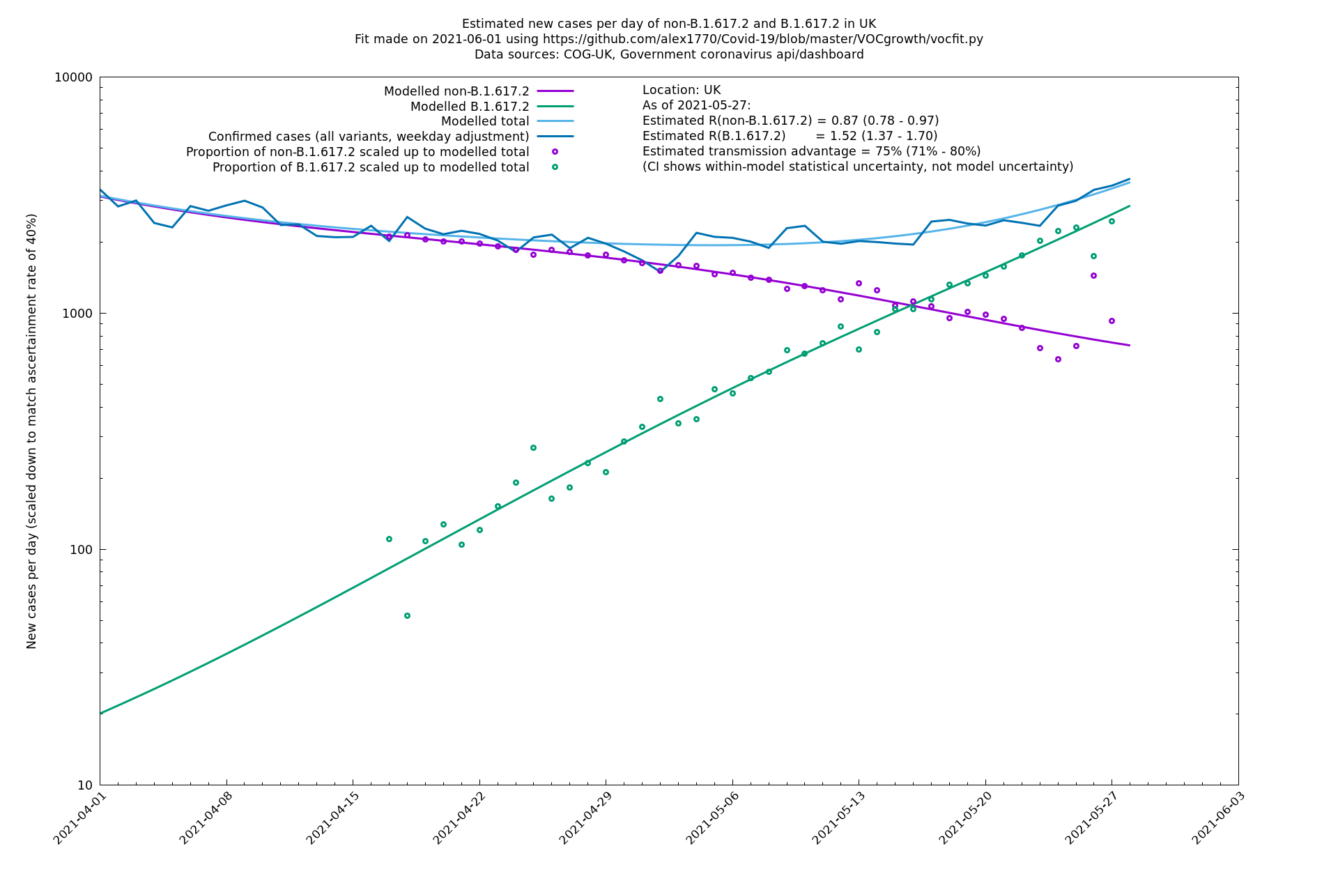
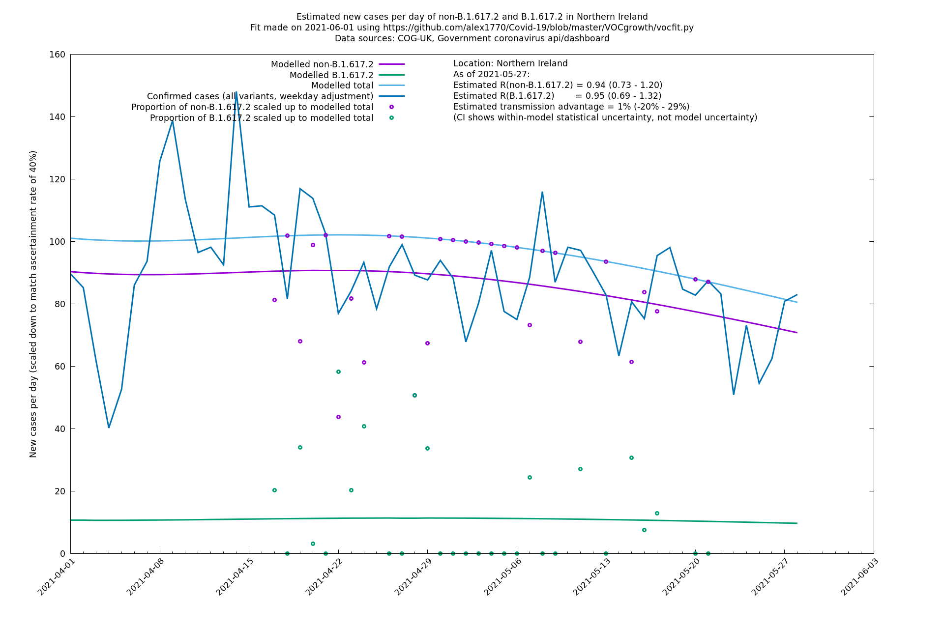
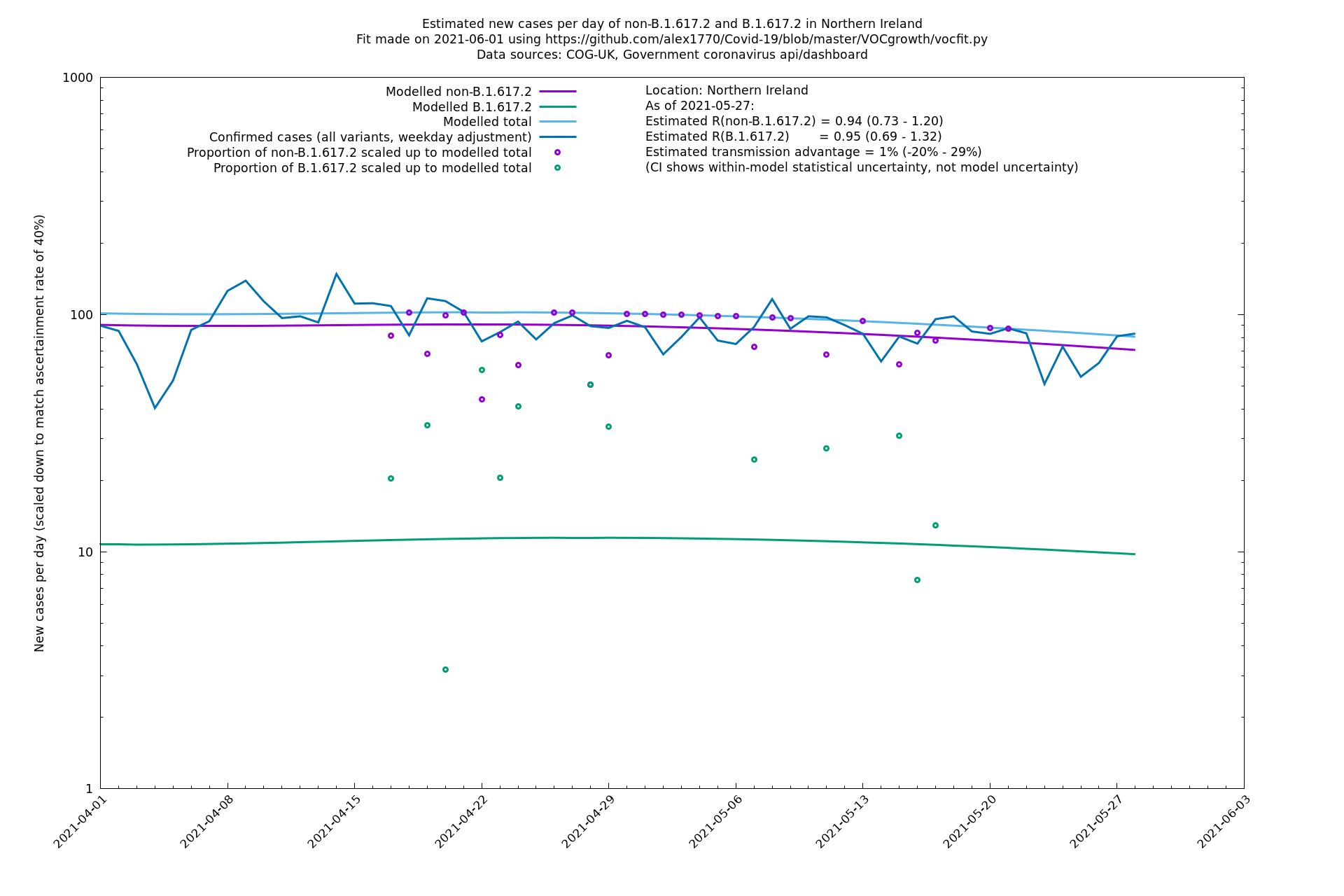
Graphical output
In each case there is a graph with a linear y-axis, followed by the same information plotted on a logarthmic scale.
If it looks like the lines are not going through the data points in the best way, then that might be because they are constrained in ways that aren't completely obvious. The two assumptions of a constant factor in transmissibility between variants, and reproduction numbers being a simple exponential of the respective growth rates, mean that the slopes of the green and purple lines in the log charts should move in tandem, a fixed difference apart.
UK using COG-UK
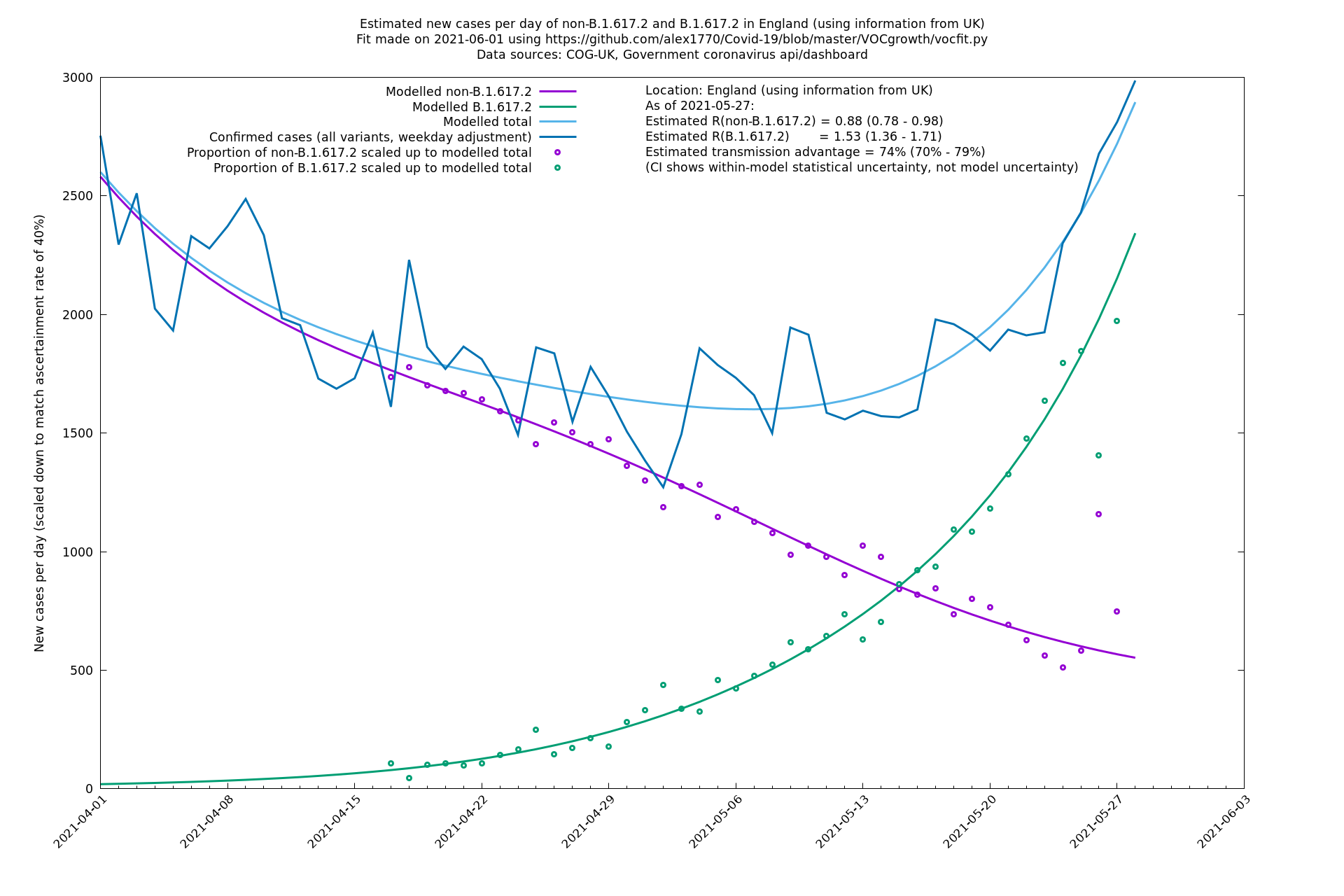
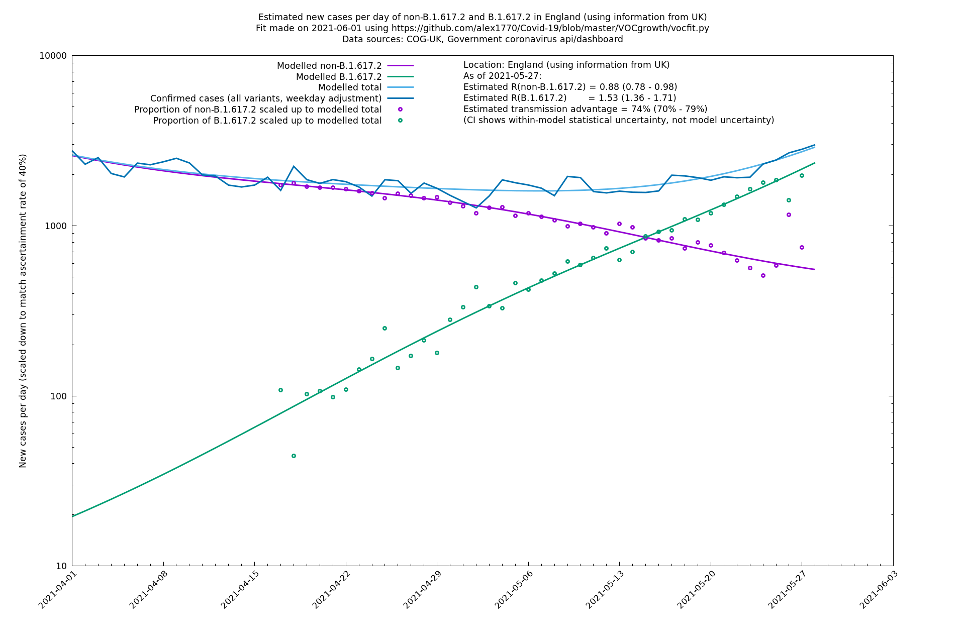
England
England is treated separately here from Scotland, Wales and Northern Ireland, because there are more data sources for it, in particular the Sanger feed which enables us to compare different ways of estimating the parameters for England.
Scotland, Wales and Northern Ireland
Bolton
Regions of England
East Midlands
East of England
London
North East
North West
South East
South West
West Midlands
Yorkshire and The Humber

Acknowledgements
I am grateful to Theo Sanderson and Tom Wenseleers for helpful conversations.