Estimating Generation Time Of Omicron

Generation Time of the Omicron Variant based on case counts in England in 2021

Alex Selby / / @alexselby1770

Abstract

There has been speculation that part of the advantage the Omicron variant has over Delta is that it has a significantly shorter generation period. It is important to establish whether or not this is the case because models of the epidemic with this as a default assumption will make substantially different predictions from those without. A shorter generation time would mean, for example, that Omicron's transmission advantage is lower than it otherwise would be which in turn would mean that restrictions (NPIs, reduction of contacts) ought to have a disproportionately successful effect on reducing spread. It would also suggest that a person's infectious period typically starts earlier and is shorter than otherwise expected, which would have implications for contact tracing and quarantine. Another consequence of a lower generation time is that we would expect the epidemic, if unmitigated by restrictions, to be over more quickly than it otherwise would be.

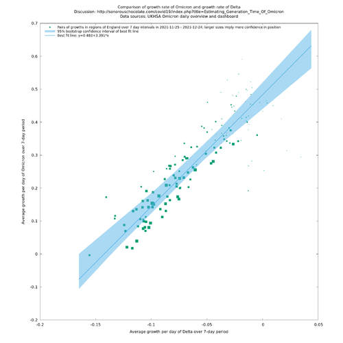
In this article we consider the sequence of Delta and Omicron daily case counts and highlight a particular striking pattern of growth in new cases per day: the daily growth rates, $$g_\Delta(t)$$ and $$g_\O(t)$$ of Delta and Omicron respectively in England from 25 November - 24 December 2021 are related to a good approximation by $$g_\O(t)=0.483+3.391g_\Delta(t)$$ (95% CI for the gradient: 2.788 - 3.663). One possible explanation for the gradient of this line being so much larger than 1 is that the generation time of Omicron is much smaller than that of Delta.

If we use the generation time distribution of Delta from Hart et al, Oct 2021, then the above linear relationship suggests that the generation time of Omicron is 46% (38% - 60%) that of Delta, or 2.12 (1.75 - 2.77) days, and that the relative transmissibility in England in December 2021, $$R_t(\O)/R_t(\Delta)$$, was 2.28 (2.03 - 2.68), lower than some early estimates that did not consider a different generation time. We then consider alternative possible explanations for the observed pattern of growth.

Note that here and throughout, confidence intervals only show statistical variation within the given model. It is possible there are larger sources of error due to an incorrect modelling assumption, as discussed in limitations below.

Linkage of growth rates and generation times

If $$\Delta_0, \Delta_1, \Delta_2, \ldots$$ and $$\O_0, \O_1, \O_2, \ldots$$ are the respective daily time series of Delta and Omicron confirmed case counts - or otherwise estimated infection numbers - in some location, then a simple model of change that assumes the variants have the same generation time and other characteristics is that they grow at respective time-varying continuous rates $$g_\Delta(t)$$ and $$g_\O(t)$$ which differ by a constant, $$h$$, say. The growth rates' time dependence is meant to account for changes in people's propensity to test, changes in case ascertainment rates (proportion of infections that are confirmed by a positive test) and changes in behaviour leading to increases or reductions in contacts, where in each case such changes are assumed to affect each variant equally. These assumptions lead to the identity $$\O_t/\Delta_t=Ce^{ht}$$ for some constant, $$C$$ and this approximation has proved successful in the past in determining the relative growth rate, $$h$$, between two variants, by simply plotting $$\log(\O_t/\Delta_t)$$ and finding the slope of (some version of) the best-fit line.

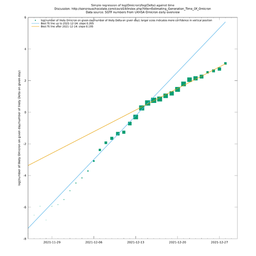
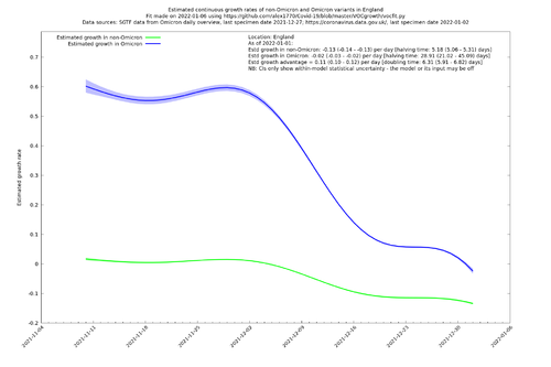
However, in past variant transitions such as Alpha-Delta in May 2021, the straight line relationship has sometimes appeared to bend over slightly as time has gone on, or otherwise slightly deviated from a single straight line. In the present case of the Delta-Omicron transition, there is a quite marked bending, as illustrated in Fig. 1 which is constructed from the ratio of estimates of Omicron to Delta on each day, using the SGTF proxy (which is known to be highly accurate for Omicron in the UK, apart from a small background rate of SGTF that is noticeable early on in Omicron's appearance, and to some extent has been adjusted for here). Fig. 2 goes a bit further and makes use of case counts in addition to variant proportions to estimate the growth rates of Delta and Omicron separately. This also suggests that $$g_\O(t)-g_\Delta(t)$$ is positively correlated with $$g_\Delta(t)$$, though case counts during the last week of December should be interpreted with more caution owing to unusual testing patterns and possible limitations of testing capacity. (Note that the analysis in Fig. 2 is just for illustration/motivation here and is not relied upon in this article.)

Fig. 1 (click to enlarge)

Fig. 2 (click to enlarge)

This effect, a positive correlation between $$g_\O(t)-g_\Delta(t)$$ and $$g_\Delta(t)$$, is what one would expect to see if Omicron's generation period were lower than Delta's. That is because instead of $$g_\O(t)-g_\Delta(t)$$ being constant, it is more natural to suppose that $$R_t(\O)/R_t(\Delta)$$ is constant: for example, if you halve the number of people you meet, then other things being equal, you are on average likely to halve the number of people you infect, which is to say, reduce $$R_t(\O)$$ or $$R_t(\Delta)$$ by the same factor. Similarly, other forms of "noise", such as changes in propensity to test, would also be expected to have a proportional effect on the apparent values of $$R_t$$. In the simplest possible approximation that allows for different generation times, we'd have $$R_t(\Delta)=e^{T_\Delta g_\Delta}$$ where $$T_\Delta$$ is the generation time of Delta, and a similar equation for Omicron, which implies $$T_\Delta g_\Delta-T_\O g_\O$$ is constant.

A linear relationship between $$g_\Delta$$ and $$g_\O$$, though with different coefficients, would still be expected to hold under slightly more general conditions, and this is what we consider in this article. The standard relationship between $$R$$, $$g$$ and generation time distribution $$T$$ is $$R\mathbb E[e^{-gT}]=1$$, and a popular and convenient family of positive distributions with two free parameters to use for $$T$$ is the Gamma family. In shape-scale notation, if $$T\sim\Gamma(k,\theta)$$, then $$R=(1+g\theta)^k$$. If we suppose $$T_\Delta$$ and $$T_\O$$ have the same shape parameter, $$k$$, then $$R_t(\O)/R_t(\Delta)$$ being constant would still lead to a linear relationship between $$g_\Delta(t)$$ and $$g_\O(t)$$. Provided we have a decently varied supply of pairs $$(g_\Delta(t),g_\O(t))$$ of reasonable quality, we should be able to discover this linear relationship, and hence get a relationship between $$k$$, $$\theta_\O$$, $$\theta_\Delta$$ and $$R_t(\O)/R_t(\Delta)$$. If we are additionally willing to make use of previously estimated values of $$\theta_\Delta$$ and $$k_\Delta$$, then we can estimate $$\theta_\O$$ and $$R_t(\O)/R_t(\Delta)$$, hence arriving at an estimate for the generation time of Omicron and its current transmission advantage over Delta.

There is no reason in principle why we can't estimate parameters in the wider situation of $$k_\O\neq k_\Delta$$, but there is a question of how much information the data is powered to yield, and trying for an extra parameter like this is probably pushing it. Furthermore, the relationship between $$g_\O$$ and $$g_\Delta$$ does look pretty linear (see Fig. 3 below), so there is probably not much advantage/justification in positing this particular extra parameter right now.

Making estimates of growth pairs

To estimate the generation time in the manner suggested above, we just collect enough examples of pairs $$(g_\Delta(t),g_\O(t))$$ and then apply some suitable inference to find the relationship, though this requires a little care as $$g_\Delta(t)$$ and $$g_\O(t)$$ are not directly measurable. In the end, the cleanest/most powerful method the author has found is to use instances of $$(\frac17\log(\Delta_{t+7}/\Delta_t), \frac17\log(\O_{t+7}/\O_t))$$, where these are taken separately over the nine regions of England, and $$t+7<\text{2021-12-25}$$. The reasons for these choices are:

• We get more statistical power, less autocorrelation, and a greater assurance that the eventual relationship is consistent, by subdividing the data over regions.
• Testing and reporting is significantly distorted from Christmas day, so it makes sense to censor at this point. We already have enough variation in $$g_\Delta$$ by then to make the inference (an inverse problem) well-posed.
• Taking a week long period reduces the danger that the errors in the estimates for each of $$g_\Delta(t)$$ and $$g_\O(t))$$ are correlated (likely positively) which would mess up the estimate. For example, using the estimates $$(\log(\Delta_{t+1}/\Delta_t), \log(\O_{t+1}/\O_t))$$ would introduce a distortion in each co-ordinate which would be strongly positively correlated with each other because testing has a dependency on the day of the week. This would tend to bias the coefficients of the inferred linear relationship between $$g_\Delta$$ and $$g_\O$$ to be more equal to each other than they should be.
• Aside from the day-of-week effect, taking the average over a longer period than 1 day reduces other systematic errors in the estimate of $$(g_\Delta(t),g_\O(t))$$, which might occur randomly, but nevertheless be correlated across variants. For example if people decide for whatever reason to do more testing on one day, then this is likely to increase both $$\Delta_t$$ and $$\O_t$$.

Another way to do this might be to subdivide over age, rather than over region of England, but it turns out this doesn't work so well with the currently available public data. More on this in the "Alternative explanations" section below.

Definition of $$\Delta_t$$ and $$\O_t$$

Let $$S^\text{raw}_-(t)$$ and $$S_+(t)$$ be the respective S-gene negative and positive counts in a given region of England (all variables here depend on the region of England, but region labels suppressed), obtained from the 31 December 2021 Omicron daily overview.

Let $$B_-$$ and $$B_+$$ be the average values of these over the period 2021-10-01 to 2021-11-09, taken to be comfortably before the onset of Omicron, but also recent enough to be representative of the current mix of variants and current testing conventions.

Let $$S_-(t)=\max(S^\text{raw}_-(t)-(B_-/B_+)S_+(t),0)$$, attempting to adjust for the background level of SGTF. In practice this adjustment only makes a noticeable difference in the early stages of Omicron, the last week in November for most areas of the country, and shouldn't make a huge difference to the overall estimates since points with low counts of $$S_\pm(t)$$ are down-weighted in the regression (see below).

Let $$C(t)$$ be the confirmed case count by specimen day $$t$$ in a particular region of the country.

Let

\[\Delta_t=C(t)\frac{S_+(t)}{S_+(t)+S_-(t)}\] \[\O_t=C(t)\frac{S_-(t)}{S_+(t)+S_-(t)}\]

Only days for which $$S_-(t)\ge5$$ and $$S_+(t)\ge5$$ are used here, to reduce the influence of travel cases and other early artefacts, and only days ($$t$$) before 2021-12-25 are used, to avoid the highly anomalous Christmas testing period.

One could think of using $$S_{\pm}(t)$$ unadjusted, i.e., $$\Delta_t=S_+(t)$$, $$\O(t)=S_-(t)$$, but it appears that tests in a particular region at a particular time are sometimes prioritised for TaqPath labs (capable of detecting SGTF) and sometimes not, so using raw $$S_+(t)$$, $$S_-(t)$$ would create a significant distortion in growth rates as defined above. For example, in the West Midlands on the 4th and 11th December 2021 there were respectively 797 and 2404 cases that had reported SGTF/S-Gene values, compared to 3057 and 3247 confirmed cases overall. That means the proportion of confirmed cases that were sent to TaqPath labs and had viable SGTF/S-gene readings went from 26% to 74% from one week to the next, nearly a factor of 3. The week-on-week change is what is relevant to the above growth rate statistics, but to make it even clearer that this phenomenon is an artefact, the corresponding proportion on 3rd December was 56%, so it dropped by more than a factor of 2 in one day to the 4th December. Note that in all these changes, the number of confirmed cases was roughly stable at around 3000 but the total SGTF/S-Gene-measured cases changed wildly, so it seems highly likely that it's the latter that is anomalous rather than the former since it's not really possible for the true number of infections to drop by a factor of 2 in one day and then change back up again the next. Furthermore, using raw counts $$\Delta_t=S_+(t)$$, $$\O(t)=S_-(t)$$ produces much worse fits in the subsequent analysis (i.e., the analogue of Fig. 3 shows a much weaker correlation).

Regression method and estimates for the generation time of Omicron

We start by writing $$(x_i,y_i)$$ for all instances of $$(\frac17\log(\Delta_{t+7}/\Delta_t), \frac17\log(\O_{t+7}/\O_t))$$ as $$t$$ ranges over allowable dates (see above), and as the region (suppressed in this notation) ranges over the nine regions of England. There are 147 such pairs.

We are in a situation where both $$x_i$$ and $$y_i$$ have statistical noise, so we have to do something beyond standard regression of $$y$$ on $$x$$ which assumes that $$x$$ is error-free. Another matter to take into account is so-called heteroscedasticity, i.e., that some values are going to be much more uncertain than others if they arise from low $$S_\pm(t)$$ counts.

Here we use approximations to variances (representing the statistical uncertainty in count values): \[\mathbb V[\log(\Delta_t)] \approx \frac{1}{C(t)}+\frac{S_-(t)}{S_+(t)(S_+(t)+S_-(t))}\] \[\mathbb V[\log(\O_t)] \approx \frac{1}{C(t)}+\frac{S_+(t)}{S_-(t)(S_+(t)+S_-(t))}\] which arise asymptotically in the Bayesian picture, if one thinks of $$C(t)$$, $$S_+(t)$$, $$S_-(t)$$ arising from independent Poissons with respective unknown parameters $$c$$, $$s_+$$ and $$s_-$$. Then, given uniform priors, the posteriors of $$c$$, $$s_+$$ and $$s_-$$ would be Gamma distributed: $$\Gamma(C(t)+1,1)$$, $$\Gamma(S_+(t)+1,1)$$, $$\Gamma(S_-(t)+1,1)$$ respectively, with $$\Gamma(k=\text{shape}, \theta=\text{scale})$$ notation, and then \[\mathbb V\left[\log\left(\frac{cs_+}{s_++s_-}\right)\right]=\frac{1}{C(t)}+\frac{S_-(t)}{S_+(t)(S_+(t)+S_-(t))}+O(C(t)^{-2})+O(S_+(t)^{-2})+O(S_-(t)^{-2}).\]

If we then assume independence in the measurement uncertainty of $$\log(\Delta_t)$$ and $$\log(\Delta_{t+7})$$, and similarly $$\log(\O_t)$$ and $$\log(\O_{t+7})$$, then we can use the above formulae to arrive at variance estimates $$(v_i,w_i)$$ for each $$(x_i,y_i)$$. The main effect of the variance term will be to downweight those early $$(x_i,y_i)$$ that arise from particularly low counts of $$S_-(t)$$.

Given these variances, we define the best-fit line linking the $$x_i$$ and $$y_i$$ to be $$y=a+bx$$, where $$a$$ and $$b$$ minimise \[E(a,b)=\frac12\sum_i\frac{(a+bx_i-y_i)^2}{w_i+b^2v_i}.\]

In the above, $$E(a,b)$$ is the sum of the variance-weighted square distance of each $$(x_i,y_i)$$ to the line $$y=a+bx$$ (so-called "element-wise weighted total least squares"). To make a principled interpretation of this procedure, it arises as the maximum likelihood line if one thinks of generating each $$(x_i,y_i)$$ by first picking a point $$(x^*_i,y^*_i)$$ uniformly on the line then choosing $$(x_i,y_i)$$ to be from a 2d-normal distribution centred on $$(x^*_i,y^*_i)$$ with variances $$(v_i,w_i)$$.

Confidence intervals are obtained using 100,000 samples from a moving-block bootstrap, where a block size, $$r$$, is fixed and sequences of $$(x_i,y_i)$$ corresponding to a particular region of the country and to consecutive days $$t, t+1, \ldots, t+r-1$$ are resampled together. Using a simple bootstrap here, where individual $$(x_i,y_i)$$ are independently resampled, would underestimate the uncertainty because the sequence $$(\frac17\log(\Delta_{t+7}/\Delta_t), \frac17\log(\O_{t+7}/\O_t))$$ has significant autocorrelation. The block length, $$r$$, was chosen conservatively to maximise the width of the confidence intervals, which turned out to be at $$r=7$$. The (adjusted) Durbin-Watson statistic on $$(\frac17\log(\Delta_{t+7}/\Delta_t), \frac17\log(\O_{t+7}/\O_t))$$, with a time difference of $$d$$ days, becomes approximately equal to 2, suggesting no autocorrelation, when $$d$$ is approximately 6, providing some degree of other assurance that a bootstrap with block size of 7 days may be adequate.

At this point we have a supply of samples of $$(a,b)$$, each representing a linear relationship between $$g_\Delta$$ and $$g_\O$$. In the next section we will combine these with estimates of characteristics of Delta to estimate characteristics of Omicron.

The paper Hart et al, Oct 2021 gives estimates for characteristics of Delta and credible intervals for those estimates, namely that the intrinsic generation time of Delta has mean 4.6 (4.0 - 5.4) days and standard deviation 3.1 (3.0 - 3.7) days.

If we assume generation times of Delta and Omicron are each Gamma distributed with a common shape parameter, then we can use the above estimate of the generation time distribution of Delta to arrive at an estimate for that of Omicron. The samples of $$(a,b)$$ representing lines $$g_\O=a+bg_\Delta$$ are matched up with the relationship $$(1+\theta_\O g_\O)^k=\rho(1+\theta_\Delta g_\Delta)^k$$, where $$\rho=R_t(\O)/R_t(\Delta)$$ is the effective transmission ratio. Values of $$a$$, $$b$$, $$\theta_\Delta$$ and $$k$$ give $$\rho=(1-a\theta_\Delta/b)^{-k}$$, $$\theta_\O=\theta_\Delta/(b-a\theta_\Delta)$$.

Note that to make confidence intervals for $$\theta_\O$$ and $$k$$ (equivalently, the mean and standard deviation of the generation time of Omicron), we are combining uncertainty in $$a$$ and $$b$$ from our bootstrap samples, with uncertainty in $$\theta_\Delta$$ and $$k$$ obtained by sampling a representative distribution of the mean and standard deviation of the generation time of Delta implied by Hart et al.

Results

Applying the above procedure leads to the estimate $$g_\O(t)=0.483+3.391g_\Delta(t)$$ (95% CI for the gradient: 2.788 - 3.663) for growth rates in England from 25 November - 24 December 2021. A scattergram of $$(x_i,y_i)$$ is shown in Fig. 3, in which the area of a green square is proportional to its inverse total variance over both co-ordinates (so the bigger squares are more important). It is visually clear that there is a good correlation here, though one has to be slightly careful because the autocorrelation in the data is effectively artificially multiplying the samples up by a factor of something like 4.

Fig. 3 (click to enlarge)

If we further use Hart et al on the characteristics of Delta in the manner described above, we arrive at characteristics of Omicron as shown in this table.

Quantity	Median (Low - High)
Mean generation time of Delta (from Hart et al)	4.631 (3.966 - 5.362)
Standard deviation of gen time of Delta (from Hart et al)	3.101 (3.000 - 3.692)
Mean generation time of Omicron	2.118 (1.745 - 2.771)
Standard deviation of gen time of Omicron	1.432 (1.174 - 2.154)
(Mean gen time Omicron)/(Mean gen time Delta)	0.456 (0.382 - 0.605)
$$R_t$$(Omicron)/$$R_t$$(Delta)	2.284 (2.026 - 2.676)

Limitations and discussion of alternative (i.e., unchanged generation time) explanations for the same observations

Bootstrap confidence intervals

Though seemingly reasonable, these are not perfectly rigorous in this situation and it is conceivable they are giving a false sense of confidence in the estimates. It may be better to replace this with a fully generative model which has a total likelihood for all observations.

Subpopulation dynamics/confounding

The model described here assumes a single homogeneous population in each region. It is possible, on the other hand, with different growth rates in different subpopulations, to have an overall (totalled over the whole population) relative growth rate of one variant compared to another to vary in time and be different from the (constant) relative growth rate of the two variants in each subpopulation. (This is effectively a continuous Simpson's paradox.) "Subpopulation" could mean those living in a particular location, those in a particular age band, or it could mean a subdivision that we don't even know about.

A toy example that assumes equal generation times for each variant, in effect assuming constant growth rate difference, shows what kind of effect is possible: letting $$n_{v,i}(t)$$ represent the number of new cases per day of variant $$v$$ (Delta or Omicron) in subpopulation $$i$$ on day $$t$$, we can assume that $$n_{v,i}(t)$$ decomposes as $$n_{v,i}(t)=n_{v,i}(0)e^{g_vt+h_i(t)}$$ where $$g_v$$ is the growth advantage of variant $$v$$, and $$h_i(t)$$ is the variant-independent growth rate in the subpopulation that represents how cautious about contacts (etc.) that subpopulation is. We have $$\frac{d}{dt}\log(n_{\O,i}(t)/n_{\Delta,i}(t))=g_\O-g_\Delta$$ for each subpopulation, but the relative growth rate of Omicron over Delta for the total over the whole population is \[\frac{d}{dt}\log\left(\frac{\sum_i n_{\O,i}(t)}{\sum_i n_{\Delta,i}(t)}\right)=g_\O-g_\Delta+\frac{\sum_i n_{\O,i}(t)\dot{h}_i(t)}{\sum_i n_{\O,i}(t)}-\frac{\sum_i n_{\Delta,i}(t)\dot{h}_i(t)}{\sum_i n_{\Delta,i}(t)}.\] In other words the "pure" relative growth rate between variants, $$g_\O-g_\Delta$$ is distorted by the difference of two convex combinations of subpopulation growth rates. The maximum distortion is the maximum difference in subpopulation growth rates, $$\max_i\dot{h}_i(t)-\min_i\dot{h}_i(t)$$. The distortion is positive if Omicron disease prevalence is better correlated with subpopulation growth rates than Delta disease prevalence is, and negative if it's the other way around.

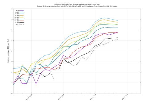
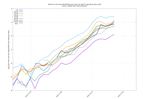
Could this mechanism explain what we are seeing here? In general it is difficult to know what is going on in all possible subpopulations, but there is some published data stratified by age and variant status, and age would be a good candidate for a relevant subpopulation division as Omicron initially had stronger growth in younger age groups, though this effect only lasted around a week (Fig. 4). A shift from "high-growth high prevalence in the young + low-growth low-prevalence in the old" to "low-growth high prevalence in the young + high-growth low-prevalence in the old" would explain the reduction in $$g_\O-g_\Delta$$, but this would require the old to become more carefree about mixing than the young, which is not impossible but not an obvious hypothesis. If stratifying by age groups deconfounded the relative growth rate in such a way as to allow for the "equal generation time" hypothesis, then we'd expect to see the relative growth of Omicron compared with Delta in each age group to form a straight line on a log scale graph ($$\frac{d}{dt}\log(n_{\O,i}(t)/n_{\Delta,i}(t))=g_\O-g_\Delta$$ in the above notation). However, Fig. 5 arguably shows a levelling-off in several individual age groups from 14 December, which wouldn't be possible if stratifying by age were sufficient to deconfound the relative growth rate. This could be clarified further if more recent age-variant data were to be published (the most recent at the time of writing being up to 18 December 2021).

Fig. 4 (click to enlarge)

Fig. 5 (click to enlarge)

Generation time itself is an approximation at many levels

The concept of generation time is in part dependent on behavioural factors: for example, more testing with rapid tests could cause people to isolate earlier which could decrease the effective infectious period. It is possible that there are different subpopulations with different levels of enthusiasm for contact-tracing which would cause different generation times for different people, but these are all mixed together and approximated as a single distribution. We then further approximate this with a particular family of distributions (Gamma), then further approximate again by supposing the shape parameter doesn't change. (On the plus side, the relationship found in Fig. 3 seems quite strong and predictive, at least over the study period, which suggests all the approximations may not be that terrible. At any rate, it seems worthwhile to give your model this extra parameter to distinguish variants.)

Unchanging relative immunity to Delta and Omicron

The assumption that the ratio $$R_\O/R_\Delta$$ is constant relies on the population's relative immunity to Omicron and Delta remaining unchanged over the course of the observed period. How close is this to being true? A full analysis is complicated and relies on knowing details of antibody waning and vaccine efficacies against the two variants, so we only propose to discuss this in broad terms here. The observed period is 25 November - 24 December 2021 and immunity to infections during that period would be generated by vaccinations and infections occurring approximately 1 week earlier, which is to say 18 November - 17 December. During that period there were about 13.2m vaccinations (mostly boosters), about 2.7m Delta infections and 0.6m Omicron infections (assuming a case ascertainment rate of 40%, as suggested by the ONS infection survey during this period). Relative to the population these are about 24%, 5% and 1% respectively. Going in the other direction is antibody waning from past infections and vaccinations, but since the period in question featured an intense vaccination campaign, the loss in immunity over this (short) period will presumably be relatively small compared to the increase in immunity. Due to the immune escape of Omicron against vaccine-induced and Delta-induced antibodies, this extra immunity will be more potent against Delta than Omicron, so will tend to decrease $$R_\Delta(t)$$ more than $$R_\O(t)$$. (There is relatively little Omicron-infection immunity over this period, and in any case there is some evidence that Omicron-induced immunity is protective against Delta.)

Note that the direction of this increased immunity is likely to diminish the effect we are seeing, which involves $$g_\O(t)$$ falling faster than $$g_\Delta(t)$$. If this change in immunity were accounted for then $$g_\Delta(t)$$ and $$g_\O(t)$$ would be revised upwards, but $$g_\Delta(t)$$ more so. In other words, if anything this is an argument in favour of a bigger generation time difference.

As for the size of the effect, 30% (24%+5%+1%) might sound like a lot, but that's the end-to-end effect. The error is more like 15% from the midpoint in the period, and it's not as much as that because a vaccination doesn't change someone from being totally susceptible to both variants to being totally susceptible to Omicron but impervious to Delta. Most vaccinations are of people who already have some degree of immunity (from infection or previous vaccination), and they are still partially effective against catching Omicron, and not totally effective against catching Delta. In summary, it seems likely that taking this effect into account would result in a small increase in the observed effect of the difference in generation times between variants.

Changes in Case Ascertainment Rate

Since the above method relies on being able to measure growth in cases from one time to another (as opposed to the ratio of cases of one variant to another), it is reliant on the ratio of confirmed cases to infections (the ascertainment rate) being roughly constant over time. Some indication that this holds is provided by the recently-published ONS infection survey prevalence estimates for London from 20 November - 31 December 2021. Up to the end of our period of study, 24 December 2021, these very closely match (a constant multiple of) the sum of the 11 days of confirmed cases by specimen date leading up to the day in question, which suggests that the ascertainment rate did not drastically change over that period in London, on a timescale of a few days or more. (Prevalence, and 11-day averaging, are blurred versions of incidence, which means it's not easy to tell from this comparison if, for example, the ascertainment rate goes up on odd days and down on even days, but we can deduce that there is agreement on a timescale of a few days or more.) Further ONS prevalence publications can be used to check the corresponding fact for other regions of the country.

AY.4.2

Away from the Omicron show, AY.4.2, a more transmissible sublineage of Delta, is slowly but surely taking over from the rest of Delta. It is approximately 10% more transmissible, but over the period 18 November - 17 December 2021, it will have only increased in prevalence from about 17% to 24% of Delta, which will have increased the overall transmissibility of Delta by about 0.7%, which is to say not very much, though it does go in the direction of slightly exaggerating the effect we are seeing ($$g_\O(t)-g_\Delta(t)$$ decreasing in time).

Conclusion

We have some unusual phenomena (Figs. 1-3), one explanation for which is that Omicron has a significantly shorter generation time than Delta. In the opinion of the author, a shorter generation time is likely to be at least part of the explanation.

Traditionally, generation times are hard to measure and require careful surveys of people's behaviour, but the above analysis suggests it might be possible to extract some information about comparative generation times between variants from simple case numbers under some circumstances, especially when it looks like the difference is large.

To do this requires a somewhat careful treatment of case counts to remove any consistent anomalous features. This is unlike simple relative growth rates, which rely on $$\log(\O_t/\Delta_t)$$ in which anomalies in $$\O_t$$ and $$\Delta_t$$ tend to cancel out nicely.

It is clear that $$g_\O(t)-g_\Delta(t)$$ being constant is not an adequate modelling assumption here as it leads to significantly wrong predictions, so something has to be added to any model that seeks to explain this Delta-Omicron transition period. And even as Delta recedes, this may still be a worthwhile exercise as the new modelling ingredient, be it a shorter generation time or something else, may survive into the Omicron era.

Program and source data

The program used is hosted on github. The above analysis was performed using commit 0f3ebb58c8.

The regional case counts were obtained from the UK government dashboard/api with this request on 3 January.

The SGTF counts were obtained from the 31 December 2021 regional data, provided by the Omicron daily overview.

Age-variant counts were obtained from the UKHSA Technical Briefing 33 (underlying data).